Introduction

In this project I explore diffusion models from both a theoretical and practical perspective. Part A focuses on working with a large pretrained model, DeepFloyd IF, to understand the forward noising process, classical and learned denoising, iterative sampling, classifier-free guidance, and image editing techniques such as SDEdit, inpainting, visual anagrams, and hybrid image synthesis. These experiments illustrate how diffusion models represent images, how noise is progressively removed, and how conditioning signals influence the generative process.

In Part B I build diffusion-inspired models from scratch on MNIST, beginning with a single-step denoiser and then extending the approach to flow matching for iterative generation. I implement time-conditioned and class-conditioned UNets, train them using the flow matching objective, and evaluate their sampling behavior over the course of training. Together, these two parts provide both a high-level understanding of diffusion-based generation and a low-level view of how such models are constructed and trained.

Part A

Part 0: Setup

In this section I use a DeepFloyd IF diffusion model to generate images. Text prompts are first produced using HuggingFace clusters and saved in a pth file. These prompts are fed into the model in two stages. The first stage produces 64x64 images, and the second stage upsamples them to 256x256. One adjustable parameter in this pipeline is the number of inference steps, which directly influences image quality by controlling how much refinement occurs during sampling.

For all experiments in Part A, I used a random seed of 67. Shown below are three prompts evaluated at two settings of the inference step count: 10 and 1000. The top row corresponds to 10 steps, and the bottom row corresponds to 1000 steps. Notice that the higher step count produces images with sharper details and more vivid colors.

Part 1: Sampling Loops

1.1 Implementing the Forward Process

Here I implement the forward process of diffusion, which takes a clean image and adds noise to it. The process is defined by \( q(x_t \mid x_0) = \mathcal{N}(x_t; \sqrt{\bar{\alpha}_t} x_0,(1 - \bar{\alpha}_t) I) \), which is equivalent to computing \( x_t = \sqrt{\bar{\alpha}_t} x_0 + \sqrt{1 - \bar{\alpha}_t}\epsilon \) where \( \epsilon \sim \mathcal{N}(0, 1) \).

The code for the forward function below shows this computation in practice. The variable alphas_cumprod stores the cumulative noise schedule for the DeepFloyd model and has length 1000, which corresponds to the number of diffusion steps.

    alpha_bar = alphas_cumprod[t]
    eps = torch.randn_like(im)
    im_noisy = alpha_bar.sqrt() * im + (1 - alpha_bar).sqrt() * eps
    

Shown below is an image of the Berkeley Campanile at different noise levels.

1.2 Classical Denoising

Next I attempt to denoise the images using classical filtering methods. A Gaussian blur is applied in an effort to reduce the noise, but the results are noticeably poor. For this experiment I used a kernel size of 15 and a sigma value of 3.

1.3 One-Step Denoising

A pretrained diffusion model is now used for denoising. The model is a UNet trained on a large dataset of noisy and clean image pairs, which allows it to estimate the Gaussian noise present in an input image. The UNet is conditioned on the amount of noise by receiving the timestep \( t \) as an additional input. Since the diffusion model was originally trained with text conditioning, I provide the text embedding for "a high quality photo" during inference.

The denoising step proceeds as follows. The noisy image \( x_t \) is passed into the UNet, which predicts the noise \( \epsilon \). This noise prediction is then removed from the noisy image using the closed-form expression \( x_0 = \frac{x_t - \sqrt{1 - \bar{\alpha}_t}\epsilon}{\sqrt{\bar{\alpha}_t}} \) to obtain a denoised image. Shown below are the results of this one-step denoising procedure. Notice that at higher levels of noise, the denoised image starts to resemble the original image less and less.

1.4 Iterative Denoising

Diffusion models are designed to denoise images iteratively. In this section I implement this process. In theory, one could start at \( t = 1000 \) and step backward one timestep at a time, but this is slow and computationally expensive. To speed up inference, we skip timesteps by using a sequence of strided values.

The array strided_timesteps specifies the timesteps used during sampling, where strided_timesteps[0] is the largest value of \( t \) and corresponds to the noisiest image, while strided_timesteps[-1] corresponds to \( t = 0 \) and represents a clean image. For this experiment I used a starting timestep of 990 with a stride of 30.

On the \( i \)-th denoising step we have \( t = \text{strided_timesteps}[i] \) and want to move to \( t' = \text{strided_timesteps}[i+1] \), which corresponds to transitioning from a noisier image to a slightly cleaner one. The update rule for producing the next image is \[ x_{t'} = \frac{\sqrt{\bar{\alpha}_{t'}}\beta_t}{1 - \bar{\alpha}_t}x_0 + \frac{\sqrt{\alpha_t}(1 - \bar{\alpha}_{t'})}{1 - \bar{\alpha}_t}x_t + v_\sigma . \] Here \( x_t \) is the noisy image at timestep \( t \), \( x_{t'} \) is the less noisy image at timestep \( t' \), \( \alpha_t = \frac{\bar{\alpha}_t}{\bar{\alpha}_{t'}} \), \( \beta_t = 1 - \alpha_t \), and \( x_0 \) is our current estimate of the clean image obtained from one-step denoising. The term \( v_\sigma \) represents additional noise, which in the DeepFloyd model, is also predicted by the network.

Shown below is a code snippet that implements the core logic of the iterative_denoise function, followed by a visualization of each iteration applied to a noisy image of the Campanile. Beneath that is a comparison between the original image, the iteratively denoised result, the one-step denoised result, and the classically filtered result. The iterative method produces the cleanest visual result, although it still does not perfectly match the original image.

    strided_timesteps = torch.linspace(990, 0, 34).long()

    alpha_bar = alphas_cumprod[t]
    alpha_bar_prime = alphas_cumprod[prev_t]
    alpha = alpha_bar / alpha_bar_prime
    beta = 1 - alpha

    x_o = (image - (1 - alpha_bar).sqrt() * noise_est) / alpha_bar.sqrt()
    term1 = alpha_bar_prime.sqrt() * beta * x_o
    term2 = alpha.sqrt() * (1 - alpha_bar_prime) * image
    pred_mean = (term1 + term2) / (1 - alpha_bar)
    pred_prev_image = add_variance(predicted_variance, t, pred_mean)
    

1.5 Diffusion Model Sampling

The iterative_denoise function can also be used to generate images from scratch. By setting i_start = 0 and initializing im_noisy with random noise, the model synthesizes an image through the full denoising trajectory. The prompt used for the five results shown below was "a high quality photo".

1.6 Classifier-Free Guidance (CFG)

As shown in the previous section, the generated images are not very high quality. They can be improved using a technique called Classifier-Free Guidance (CFG). In CFG, we compute both a conditional and an unconditional noise estimate, denoted \( \epsilon_c \) and \( \epsilon_u \) respectively. The final noise estimate is then \[ \epsilon = \epsilon_u + \gamma(\epsilon_c - \epsilon_u), \] where \( \gamma \) controls the strength of the guidance. When \( \gamma = 0 \), the model produces an unconditional estimate. When \( \gamma = 1 \), the estimate is fully conditional. Higher quality samples are typically obtained when \( \gamma > 1 \).

In this section I implement the iterative_denoise_cfg function, which extends the earlier iterative_denoise method by incorporating CFG. To obtain the unconditional noise estimate, I pass an empty prompt embedding corresponding to the null prompt "". The code snippet below shows the modifications needed to apply CFG during iterative denoising. Following that are five sampled images generated with \( \gamma = 7 \).

    cfg_noise_est = uncond_noise_est + scale * (noise_est - uncond_noise_est)

    x_o = (image - (1 - alpha_bar).sqrt() * cfg_noise_est) / alpha_bar.sqrt()
    

1.7.0 Image-to-image Translation

In this section I experiment with taking the original Campanile image, adding a small amount of noise, and then projecting it back onto the manifold of natural images without any text conditioning. This allows us to make controllable edits to an existing image, where adding more noise leads to larger edits. The idea works because denoising requires the diffusion model to infer missing details, which gives it the ability to hallucinate plausible structure. This process produces an image that is similar to the original in overall content but altered in a way that depends on the noise level. This follows the principles of the SDEdit algorithm.

The procedure is implemented by first applying the forward function to add noise to the Campanile image, then running iterative_denoise_cfg with different starting indices in strided_timesteps to denoise it. The results are shown below. Images that start closer to the original (with less noise) remain more faithful, while those that begin from heavy noise eventually resemble random samples and retain little structure from the input image.

Shown below are edits of two additional test images of my own, produced using the same procedure.

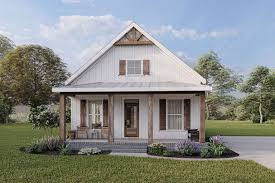
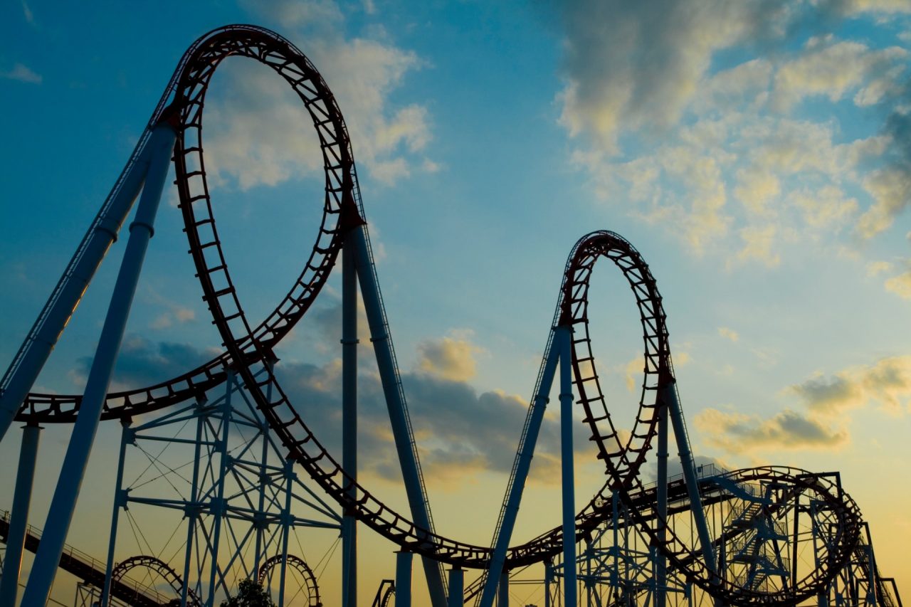
1.7.1 Editing Hand-Drawn and Web Images

I then apply this procedure to non-realistic images to project them onto the natural image manifold. Shown below are three examples.

1.7.2 Inpainting

The same procedure can be used to implement inpainting. Given an image \( x_{\text{orig}} \) and a binary mask \( m \), the goal is to produce a new image that preserves the original content where \( m = 0 \) and generates new content where \( m = 1 \).

To accomplish this, the CFG diffusion denoising loop is run as usual, but at every step we overwrite the unmasked regions of \( x_t \) with the noisy version of the original image. More precisely, after computing \( x_t \) we apply \[ x_t \leftarrow mx_t + (1 - m)\text{forward}(x_{\text{orig}}, t). \] This ensures that the unmasked pixels remain fixed while the masked region is regenerated by the diffusion model.

Shown below are the relevant modifications to iterative_denoise_cfg needed to perform inpainting. Following that are three sets of results, each displaying the original image, the mask, the masked input, and the final inpainted output. Because inpainting is a task the diffusion model was not trained for, several sampling attempts were needed to obtain clean and visually consistent results.

    pred_prev_image = mask * pred_prev_image + (1 - mask) * forward(original_image, prev_t)
    

1.7.3 Text-Conditional Image-to-image Translation

Here I apply the same procedure as in Section 1.7.0, similar to SDEdit, but now guide the projection using a text prompt. The conditional prompt is no longer fixed to "a high quality photo" and can be replaced with any prompt of my choosing. Shown below are edits of the Campanile and two additional test images using custom conditional prompts.

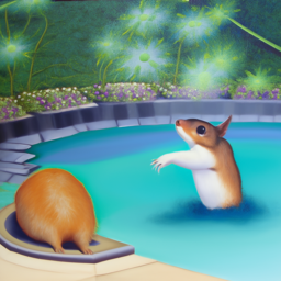
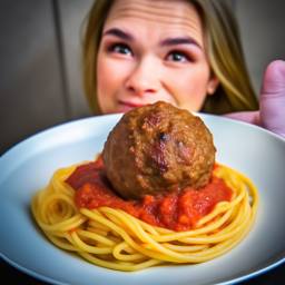
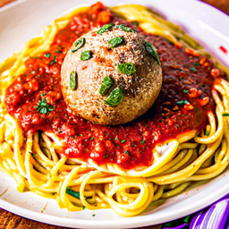
1.8 Visual Anagrams

Here I implement visual anagrams to create optical illusions with diffusion models. The goal is to generate an image that appears as one concept when viewed upright and as a different concept when viewed upside down.

To accomplish this, the image \( x_t \) is denoised at timestep \( t \) using prompt \( p_1 \) to produce a noise estimate \( \epsilon_1 \). The same image is then flipped upside down and denoised with prompt \( p_2 \) to produce \( \epsilon_2 \). After obtaining these estimates, I flip \( \epsilon_2 \) back to the original orientation, apply CFG to both, and then average them to obtain the final noise estimate \( \epsilon \). More succinctly, \[ \epsilon_1 = \text{CFG of UNet}(x_t, t, p_1) \] \[ \epsilon_2 = \text{flip}(\text{CFG of UNet}(\text{flip}(x_t), t, p_2)) \] \[ \epsilon = \frac{\epsilon_1 + \epsilon_2}{2} \] Note that for this section and all sections that follow, two conditional prompts are used, which produces two predicted variances. I chose to average these variances to get the overall predicted variance.

Shown below are the relevant modifications to iterative_denoise_cfg needed to implement the visual_anagrams function, along with two visual anagrams I was able to generate. The prompts I used were, "upright sword centered, polished metal blade", "upright candle centered, warm glowing flame", "a lithography of a standing human figure, arms raised, centered silhouette background", and "a lithography of a bare symmetrical tree, centered silhouette on plain background".

    image = torch.randn((1, 3, 64, 64), device=device).half()

    noise_est1, predicted_variance1 = torch.split(model_output_1, image.shape[1], dim=1)
    noise_est2, predicted_variance2 = torch.split(model_output_2, image.shape[1], dim=1)
    uncond_noise_est, _ = torch.split(uncond_model_output, image.shape[1], dim=1)
    predicted_variance = (predicted_variance1 + predicted_variance2) / 2

    noise_est2 = TF.vflip(noise_est2)

    cfg_noise_est1 = uncond_noise_est + scale * (noise_est1 - uncond_noise_est)
    cfg_noise_est2 = uncond_noise_est + scale * (noise_est2 - uncond_noise_est)
    cfg_noise_est = (cfg_noise_est1 + cfg_noise_est2) / 2
    

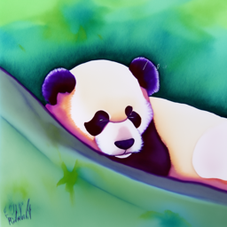
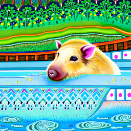
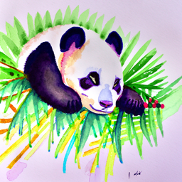
1.9 Hybrid Images

Here I implement factorized diffusion to create hybrid images. In this approach, the composite noise estimate \( \epsilon \) is constructed by predicting noise using two different text prompts and then combining the low frequencies from one estimate with the high frequencies from the other. \[ \epsilon_1 = \text{CFG of UNet}(x_t, t, p_1) \] \[ \epsilon_2 = \text{CFG of UNet}(x_t, t, p_2) \] \[ \epsilon = f_{\text{lowpass}}(\epsilon_1) + f_{\text{highpass}}(\epsilon_2) \]

Shown below are the relevant modifications to iterative_denoise_cfg needed to implement the make_hybrids function, followed by three hybrid images I was able to generate. The prompts I used were "oil painting style, a panda", "oil painting style, a canyon", "a lithography of a skull", "a lithography of waterfalls", "a watercolor of a panda", and "a watercolor of a library". For the filtering step, I used a kernel size of 33 and a sigma value of 2.

    image = torch.randn((1, 3, 64, 64), device=device).half()

    noise_est1, predicted_variance1 = torch.split(model_output_1, image.shape[1], dim=1)
    noise_est2, predicted_variance2 = torch.split(model_output_2, image.shape[1], dim=1)
    uncond_noise_est, _ = torch.split(uncond_model_output, image.shape[1], dim=1)
    predicted_variance = (predicted_variance1 + predicted_variance2) / 2

    cfg_noise_est1 = uncond_noise_est + scale * (noise_est1 - uncond_noise_est)
    cfg_noise_est2 = uncond_noise_est + scale * (noise_est2 - uncond_noise_est)

    low_est1 = TF.gaussian_blur(cfg_noise_est1, kernel_size, sigma)
    high_est2 = cfg_noise_est2 - TF.gaussian_blur(cfg_noise_est2, kernel_size, sigma)
    cfg_noise_est = low_est1 + high_est2
    

Part B

Part 1: Training a Single-Step Denoising UNet

1.1 Implementing the UNet

Here I start by building a simple one-step denoiser. Given a noisy image \( z \), the goal is to train a denoiser \( D_{\theta} \) that maps \( z \) to its corresponding clean image \( x \). To do this, we optimize an L2 objective, \[ L = \mathbb{E}_{z, x} \lVert D_{\theta}(z) - x \rVert^{2}. \] The model architecture is shown below. It consists of a sequence of downsampling and upsampling blocks with skip connections. These skip connections help the model retain high-frequency information and prevent it from discarding details from the input image. In the diagrams, \( D \) denotes the number of hidden channels, which is a tunable hyperparameter.

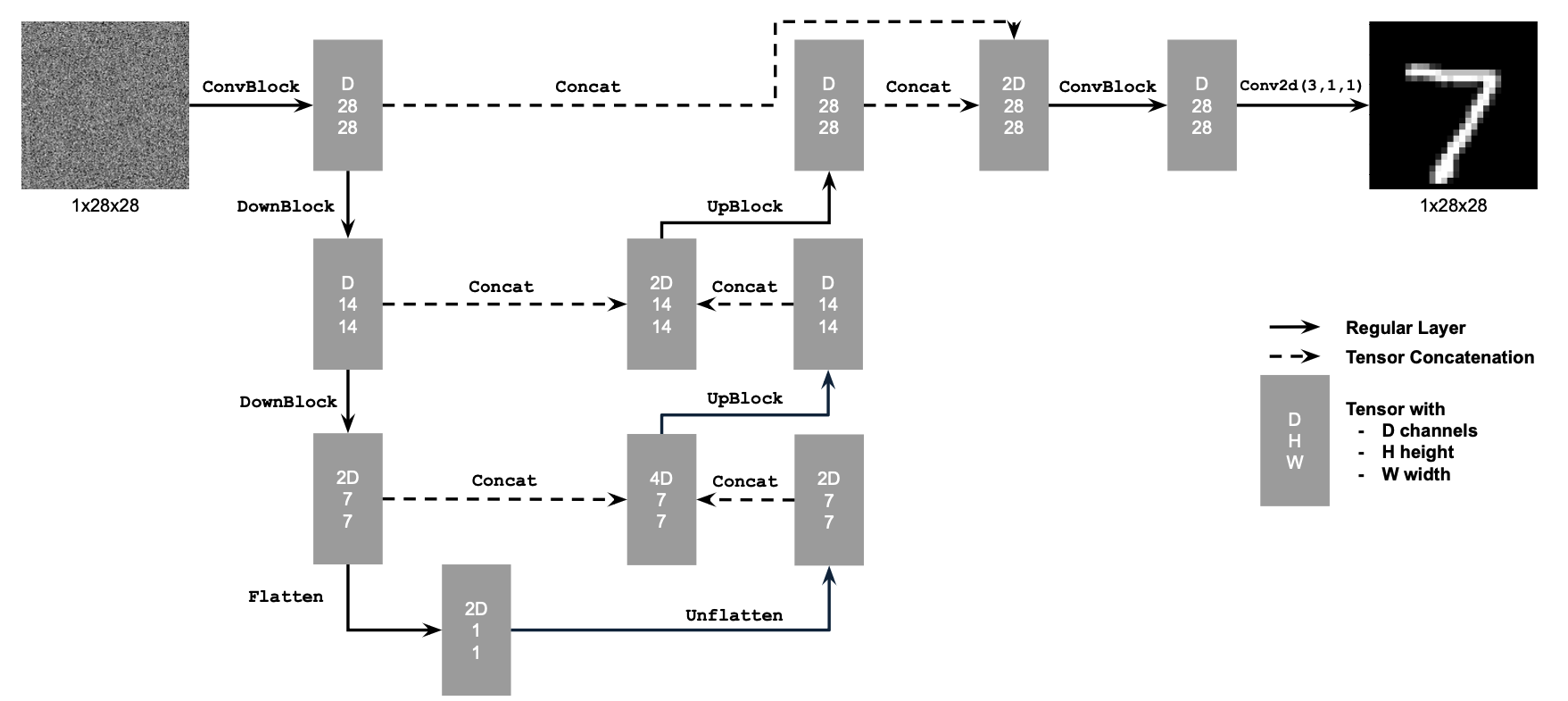
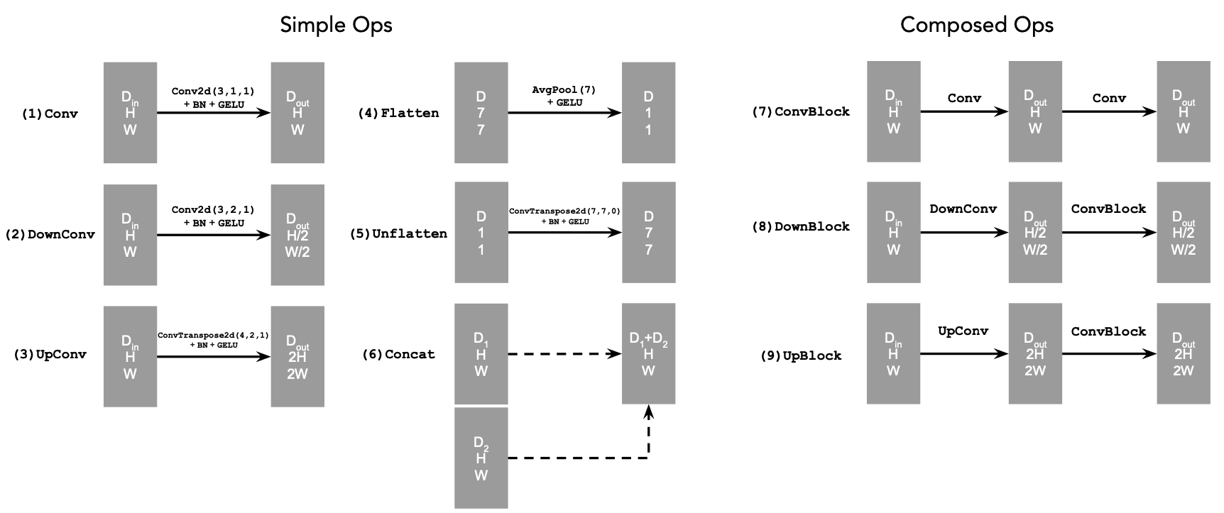
At a high level, the Conv blocks increase the number of channels, the DownConv blocks downsample the tensors by a factor of 2, and the UpConv blocks upsample them by a factor of 2. The Flatten layer performs average pooling to convert a 7x7 tensor into a 1x1 tensor, while the Unflatten layer reverses this operation by expanding a 1x1 tensor back into a 7x7 tensor. Finally, Concat represents channel-wise concatenation between two tensors of the same spatial size.

1.2 Using the UNet to Train a Denoiser

To train the denoiser UNet, we need to generate training pairs \( (z, x) \) where each \( x \) is a clean MNIST digit and each \( z \) is a noisy version of the clean image. We construct the noisy image \( z \) using \[ z = x + \sigma \epsilon, \qquad \epsilon \sim \mathcal{N}(0, I). \] Shown below is a visualization of the noise process for \( \sigma \in [0.0, 0.2, 0.4, 0.5, 0.6, 0.8, 1.0] \), assuming the clean images \( x \in [0, 1] \) are normalized. As \( \sigma \) increases, the images become progressively noisier until the original digit is no longer recognizable.

1.2.1 Training

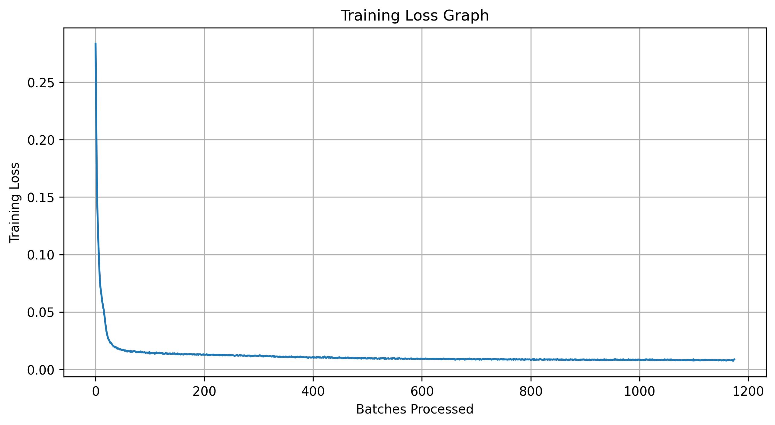
Now I train the model to perform denoising. For this experiment I set \( \sigma = 0.5 \) and use the MNIST dataset via torchvision.datasets.MNIST. The training setup uses a batch size of 256, 5 epochs, a hidden dimension of \( D = 128 \), and the Adam optimizer with a learning rate of 1e-4. Noise is added on the fly when batches are fetched from the dataloader, so each epoch presents the network with newly noised images due to the fresh samples of \( \epsilon \). This improves generalization by preventing the model from memorizing fixed noise patterns.

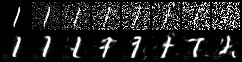
Shown below are the results of training. After the first and fifth epochs, three MNIST digits are sampled, noised, and then denoised using the model. The corresponding outputs are displayed, along with a plot of the training loss.

1.2.2 Out-of-Distribution Testing

The denoiser was trained on MNIST digits noised with \( \sigma = 0.5 \). Shown below are its results on a range of noise levels it was not trained for, specifically \( \sigma \in [0.0, 0.2, 0.4, 0.5, 0.6, 0.8, 1.0] \). For noise levels below 0.5, the model generally produces clean and recognizable digits, although there is occasional ambiguity between similar classes (for example, 1 and 7). For noise levels above 0.5, the model is no longer able to remove the noise effectively, and the outputs typically fail to form coherent digits.

1.2.3 Denoising Pure Noise

To make denoising a generative task, we would like the model to denoise pure Gaussian noise. In this setting, we begin with a blank canvas \( z = \epsilon \) where \( \epsilon \sim \mathcal{N}(0, I) \), and the goal is for the network to map this noise to a clean image \( x \).

The same training procedure used in Section 1.2.1 is repeated, but now the input consists solely of pure noise, which the model attempts to denoise over the course of 5 epochs. Shown below are the results of this training process. After the first and fifth epochs, three noise samples are drawn, passed through the model, and the corresponding denoised outputs are displayed. A plot of the training loss is also included.

Notice that all of the outputs look largely the same. Since the model has no information about what the original image should be, it attempts to produce an output that minimizes the expected error across all possible MNIST digits. This leads to a blurred, averaged-looking result that does not resemble any specific digit.

Part 2: Training a Flow Matching Model

In the previous sections, we saw that one-step denoising does not work well for generative tasks. To address this, we now perform iterative denoising using flow matching. The idea is to train a UNet to predict the flow that moves a noisy sample toward a clean sample. In this setup, we draw a pure noise image \( x_0 \sim \mathcal{N}(0, I) \) and aim to generate a realistic image \( x_1 \).

For iterative denoising, we need to define how intermediate noisy samples are constructed. The simplest approach, and the one used here, is linear interpolation between the noisy image \( x_0 \) and a clean training image \( x_1 \). This gives \[ x_t = (1 - t)x_0 + t x_1, \qquad x_0 \sim \mathcal{N}(0, I), t \in [0, 1]. \] This defines a vector field describing the position of a point \( x_t \) at time \( t \) as it moves from the noisy distribution \( p_0(x_0) \) toward the clean distribution \( p_1(x_1) \). The corresponding flow, which can be interpreted as the velocity of this vector field, is \[ u(x_t, t) = \frac{d}{dt} x_t = x_1 - x_0. \] Our goal is to learn a UNet \( u_{\theta}(x_t, t) \) that approximates this flow, predicting the direction in which \( x_t \) should move to reach the clean image. This leads to the following learning objective: \[ L = \mathbb{E}_{x_0 \sim p_0(x_0), x_1 \sim p_1(x_1), t \sim U[0,1]} \bigl\lVert (x_1 - x_0) - u_{\theta}(x_t, t) \bigr\rVert^{2}. \]

2.1 Adding Time Conditioning to UNet

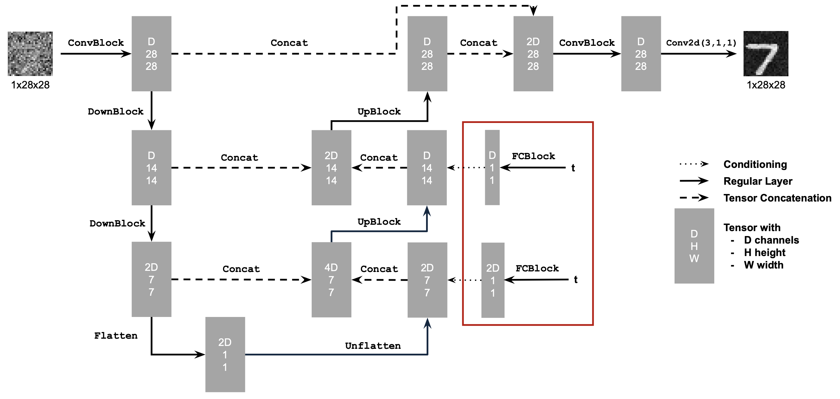
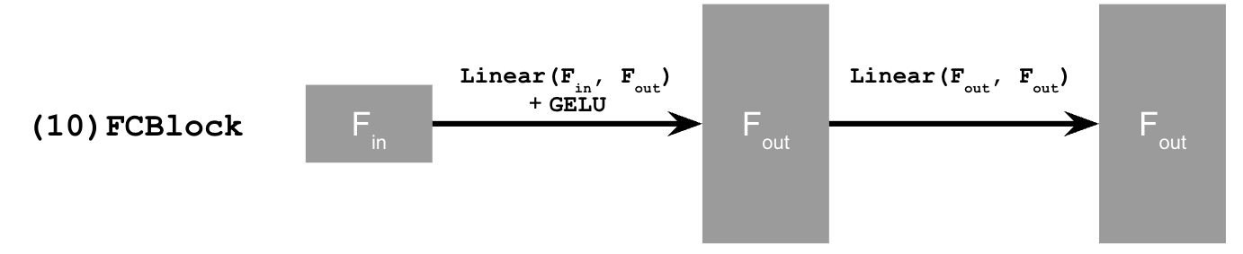
The model is now modified so that, in addition to receiving an image to denoise, it also takes a time input \( t \). To incorporate this conditioning signal into the UNet, a new module called FCBlock is added. This block processes the scalar \( t \) and produces conditioning values that are injected into the UNet by multiplying them with intermediate feature representations.

Shown below is the resulting architecture with time conditioning included and the new operation.

2.2 Training the UNet

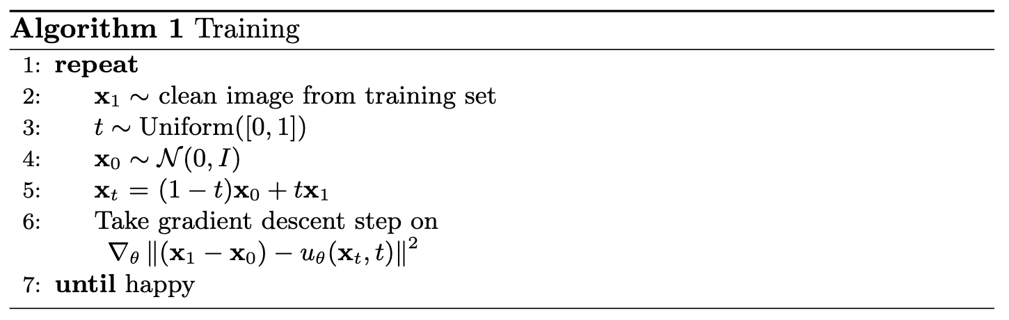
Training follows the same general procedure as before. A random clean image \( x_1 \) is sampled from the dataset, a random timestep \( t \) is drawn, noise is added to construct \( x_t \), and the UNet is trained to predict the corresponding flow at \( x_t \). This process is repeated across different images and timesteps until the model converges.

For this experiment, the batch size is set to 64 and the number of epochs is increased to 10. The hidden dimension is \( 64 \), and the Adam optimizer is used with an initial learning rate of 1e-2. An exponential learning rate decay scheduler with decay factor \( 0.1^{1.0 / \text{num\_epochs}} \) is applied, and scheduler.step() is called after every epoch.

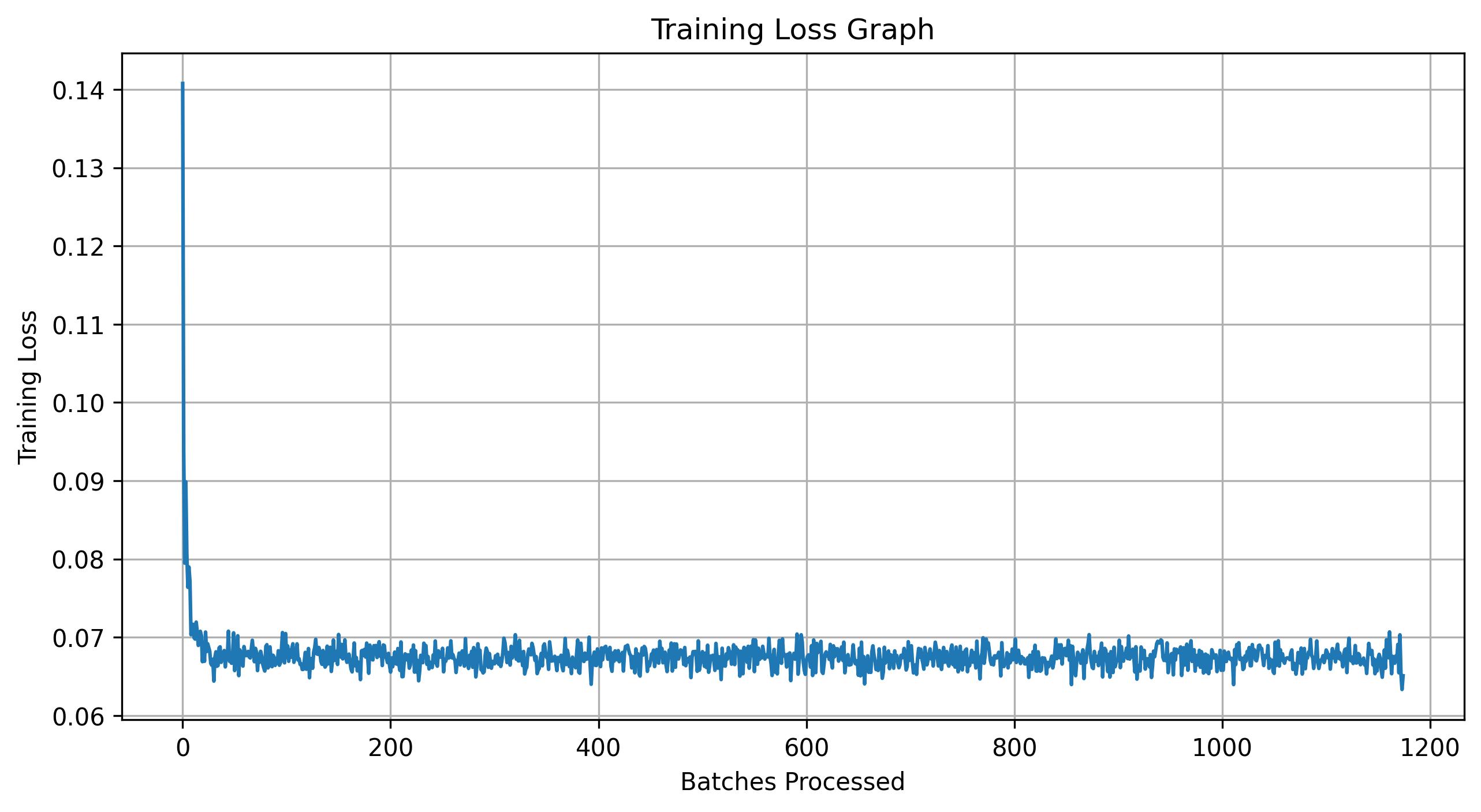
Shown below is the training algorithm and a plot of the training loss.

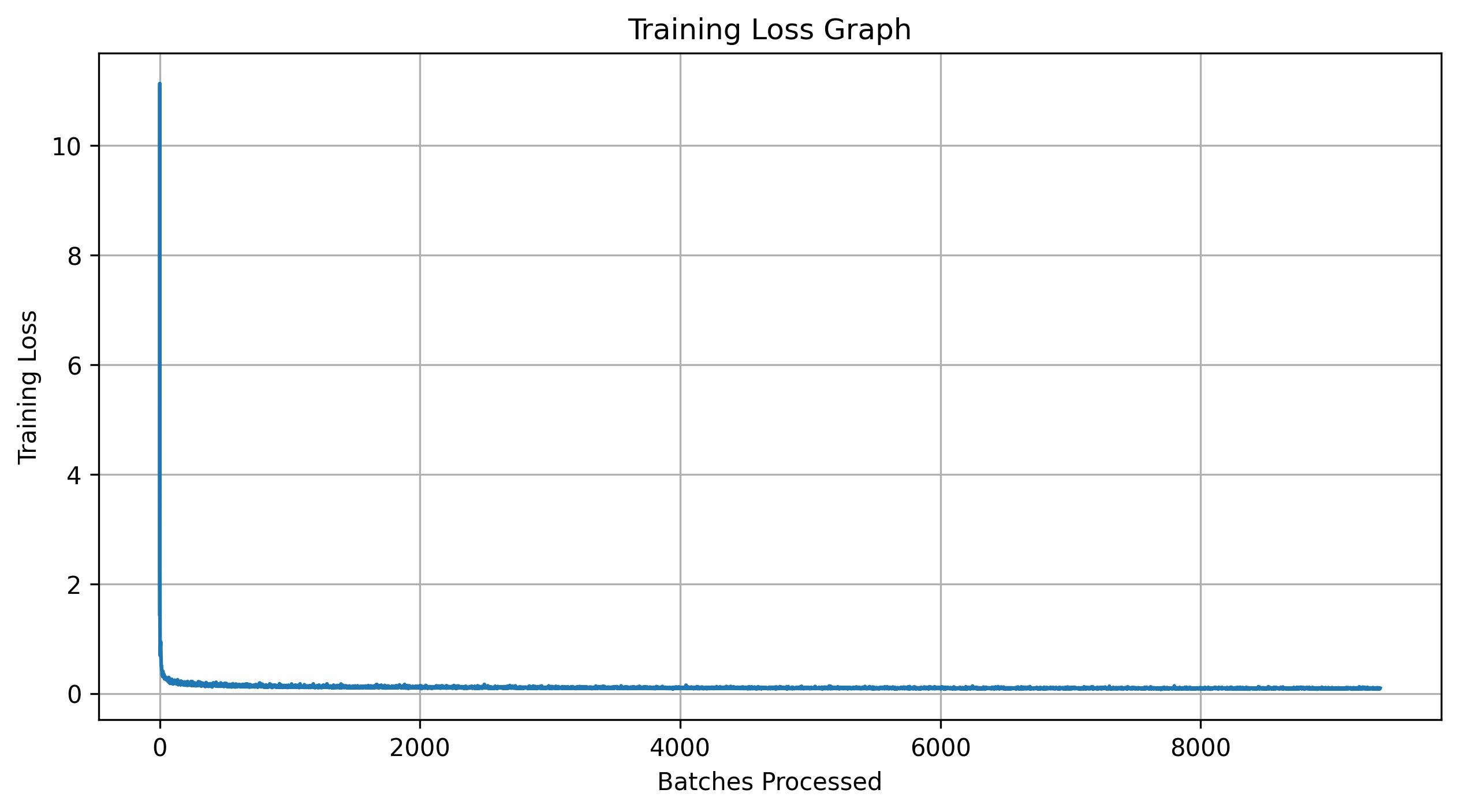
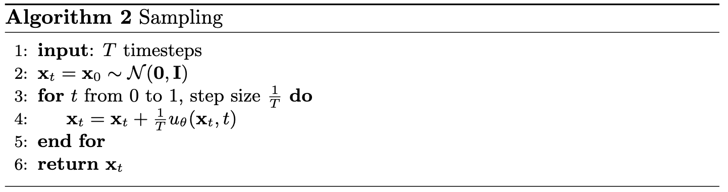
2.3 Sampling from the UNet

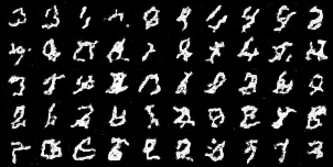
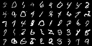
The trained UNet for iterative denoising can now be used to generate samples. Shown below is the sampling algorithm along with results after 1, 5, and 10 epochs of training. Early in training, the outputs are not recognizable, but by the final epoch, coherent digits begin to appear.

2.4 Adding Class-Conditioning to UNet

To improve generation quality and provide control over which digit is produced, we can optionally condition the UNet on the class label 0-9. This requires adding two additional FCBlock modules to the architecture and one-hot encoding the class label \( c \) into a vector that is passed through these blocks.

Because we still want the UNet to function without class conditioning, we apply dropout to the class embedding. With probability \( p_{\text{uncond}} = 0.1 \), the class conditioning vector \( c \) is replaced with zeros. Inside the model, the embedded class signal is multiplied with intermediate representations and then added to the embedded time signal.

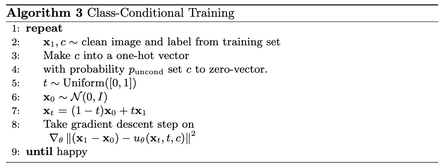
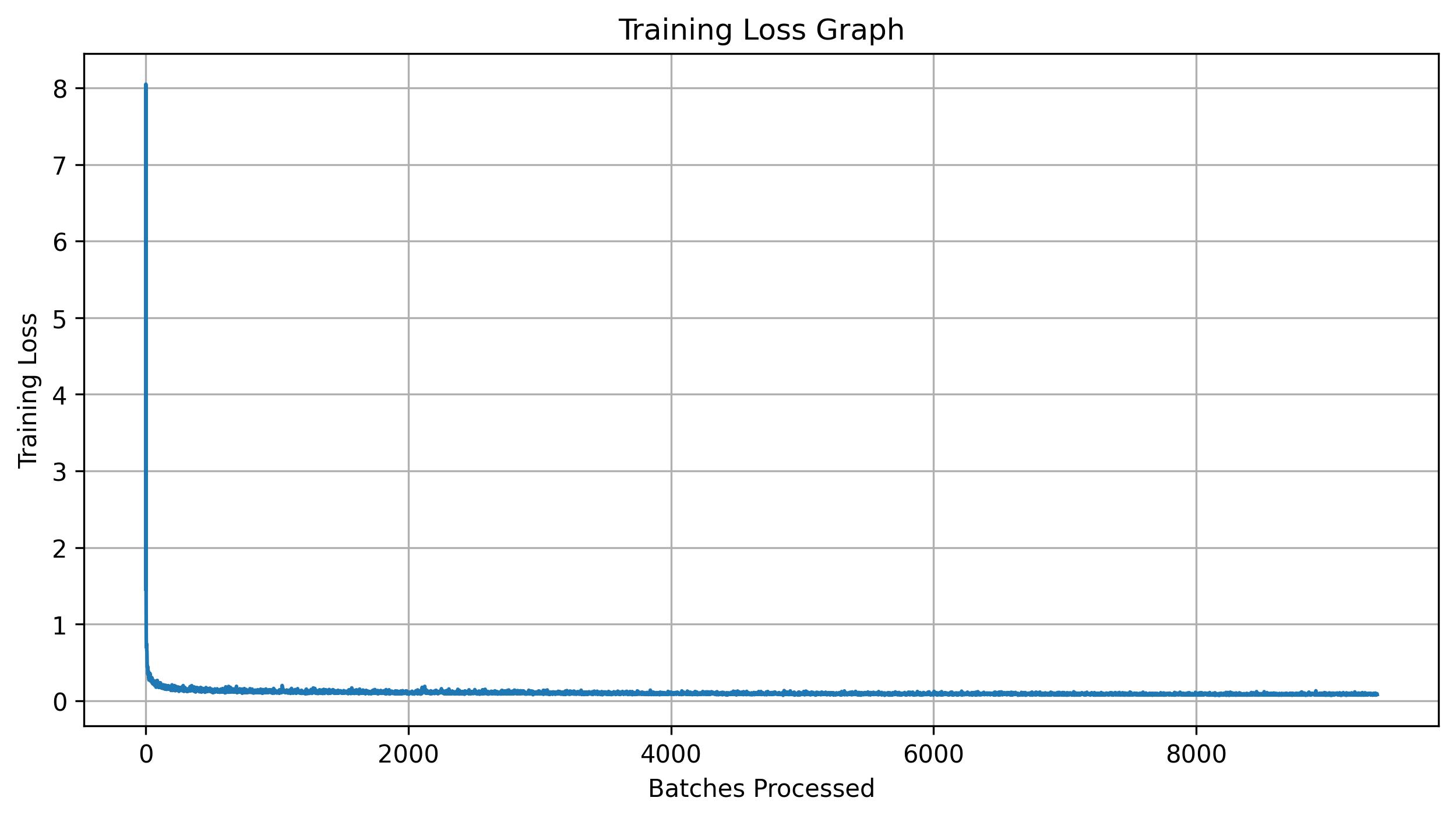
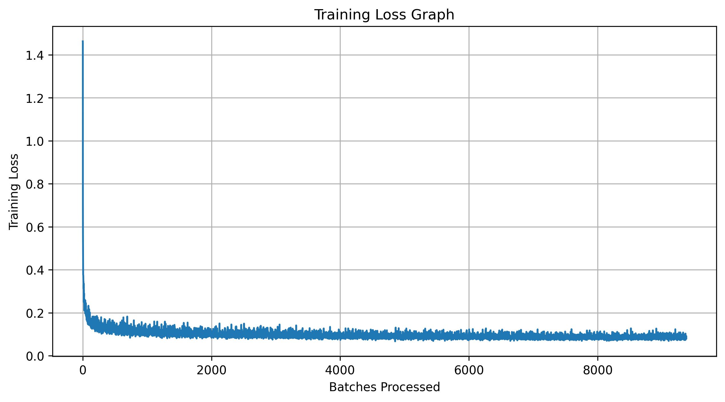
2.5 Training the UNet

Training follows the same procedure as in the previous sections, and all hyperparameters remain the same. Shown below are the training algorithm for this class-conditional UNet and a plot of the training loss for this model.

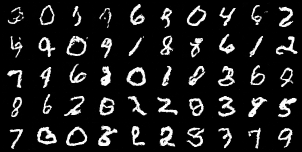
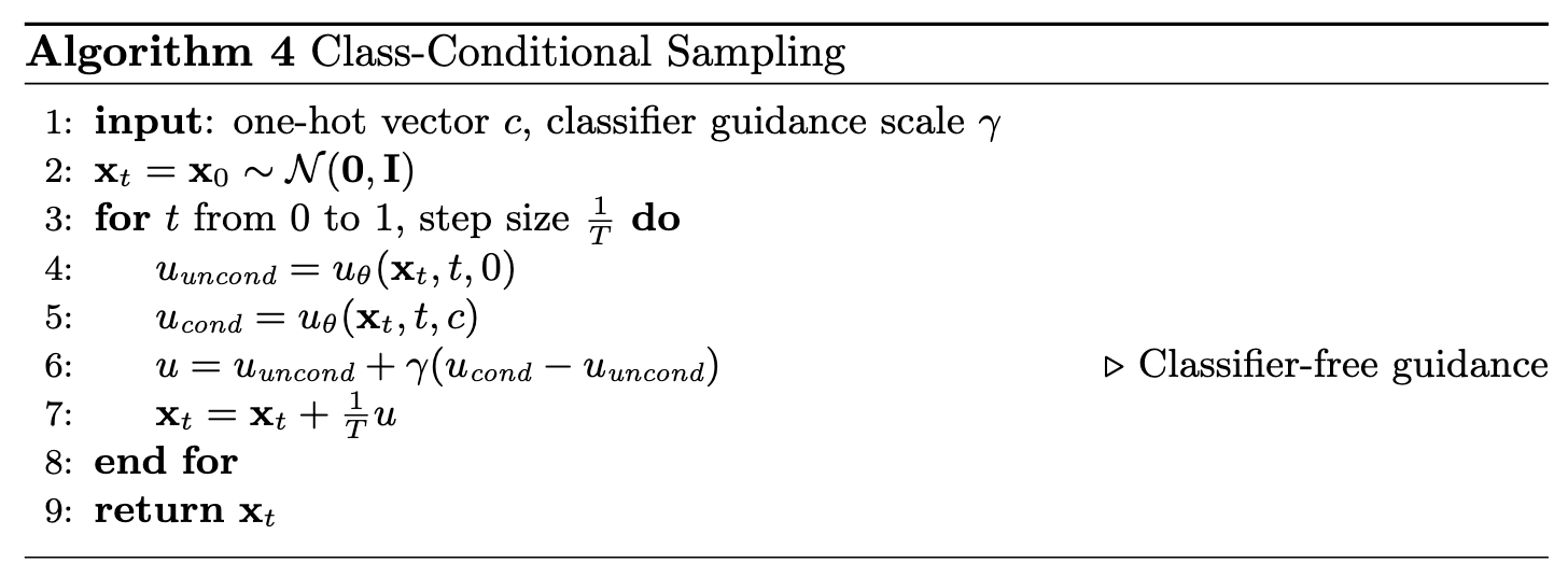
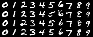
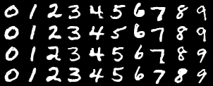
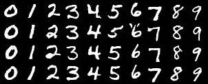
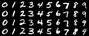
2.6 Sampling from the UNet

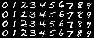
Sampling is performed using the algorithm shown below with a classifier-free guidance value of \( \gamma = 0.5 \). Shown beneath are four samples for each digit after 1, 5, and 10 epochs of training. By the final epoch, the generated digits closely resemble real MNIST samples while still remaining distinct from one another.

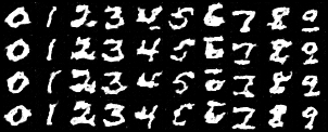
Can we remove the learning rate scheduler? The answer is yes. Without the scheduler, the learning rate no longer decays, so the original value of 1e-2 is too large for stable training. To compensate, I reduce the learning rate to 1e-3 while keeping all other parameters the same. Shown below is the training loss curve with this adjusted learning rate, along with the corresponding sampling results.