CS 180 Project 4: Neural Radiance Fields!

Introduction

This project explores Neural Radiance Fields, a method for reconstructing three-dimensional scenes from multi-view images using a fully connected neural network and volumetric rendering. The assignment begins with camera calibration and structured data capture, establishing the geometric foundations needed to recover accurate camera poses. A simple two-dimensional neural field is then implemented to build intuition for positional encoding and coordinate-based MLPs. Finally, these components are extended to a full NeRF pipeline that generates novel-view renderings of both a provided multiview dataset and a custom-captured object.

Part 0: Calibrating Your Camera and Capturing a 3D Scan

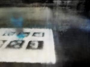
For the first part of this project, I captured a set of images to calibrate my camera and build a NeRF of my object. ArUco tags were used as visual tracking targets, providing a reliable way to detect the same 3D keypoints across different images.

Part 0.1: Calibrating Your Camera

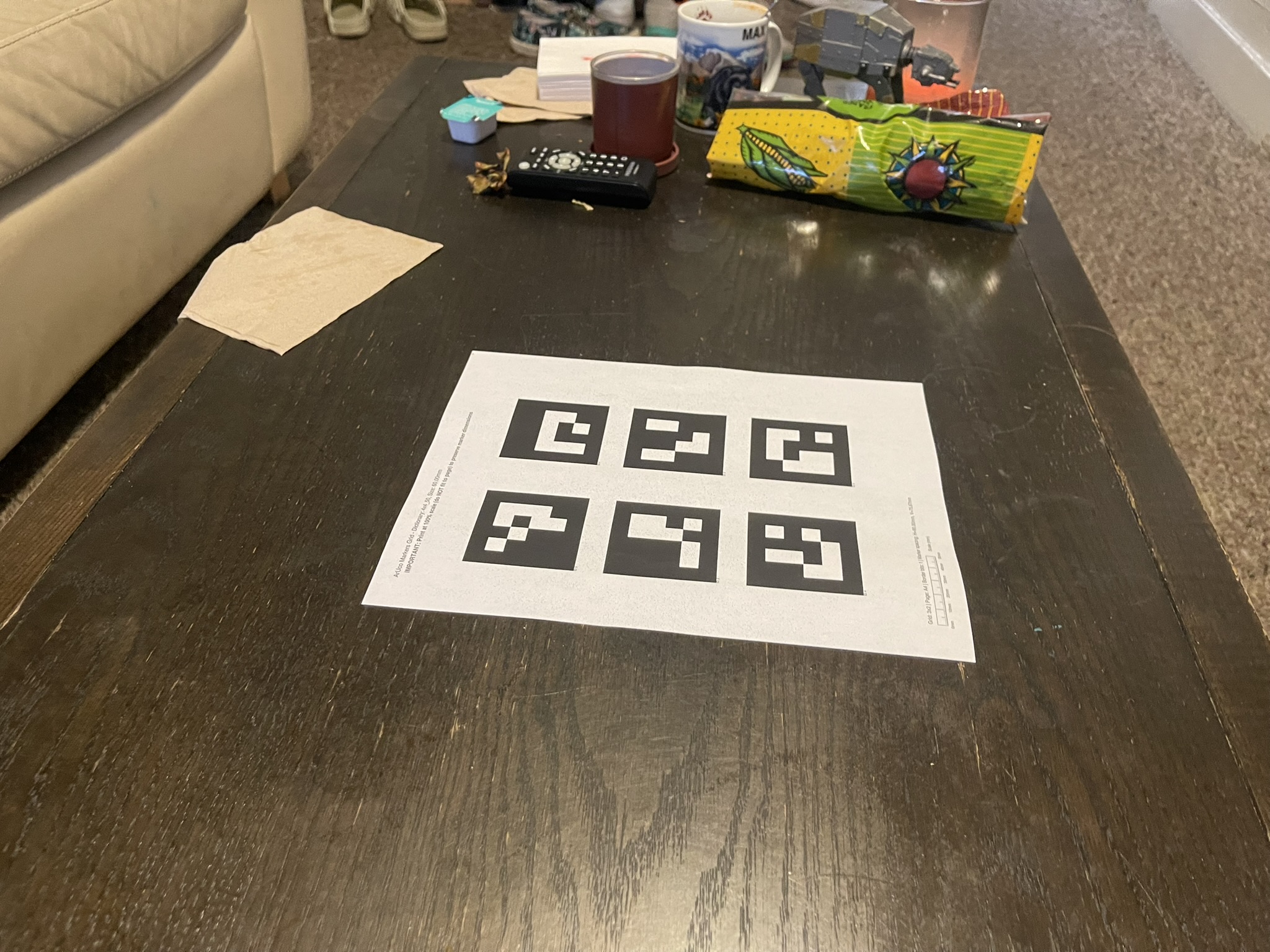
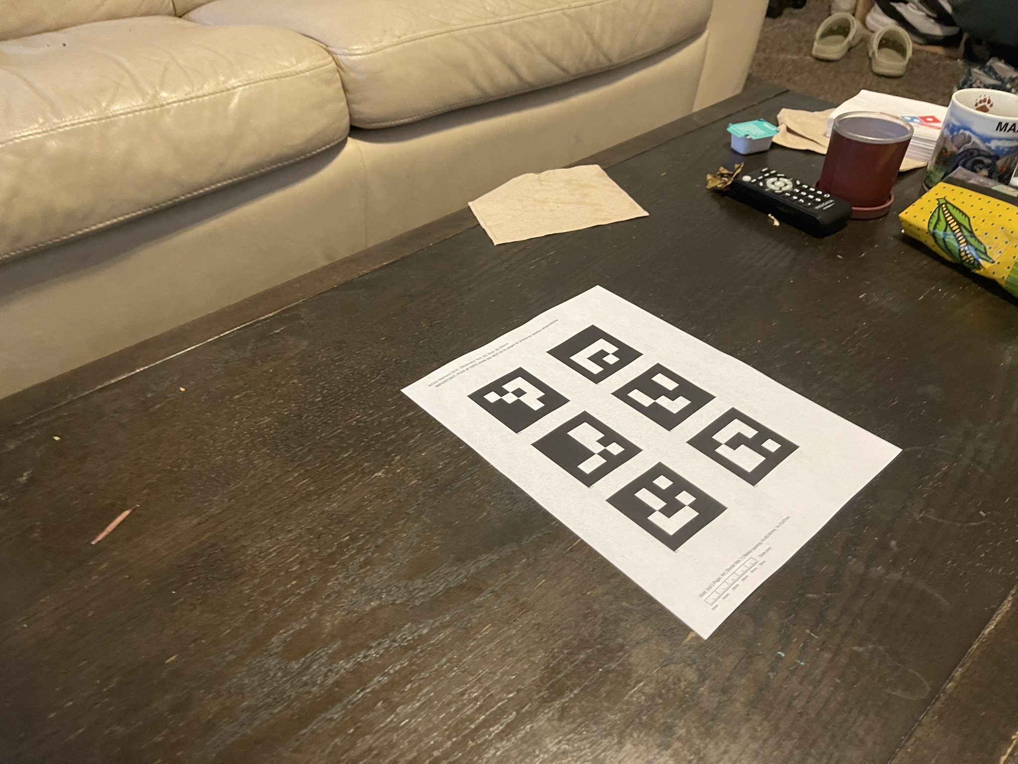
I captured approximately fifty images of the calibration tags from different viewpoints on a table. Each image was processed by detecting the tag corners and associating them with their corresponding three-dimensional world coordinates. Because the calibration tag measured 60 mm by 60 mm, I defined the corner coordinates as \((0, 0, 0)\), \((0.06, 0, 0)\), \((0.06, 0.06, 0)\), and \((0, 0.06, 0)\). These coordinates ended up being slightly different when I did my custom object as I printed an A4 document on a US Letter sized paper.

The calibration step uses cv.calibrateCamera() to estimate the camera intrinsics, specifically the camera matrix and distortion coefficients. The function receives a list of object points that describe the three-dimensional corner positions and a list of image points that correspond to the detected two-dimensional corner projections.

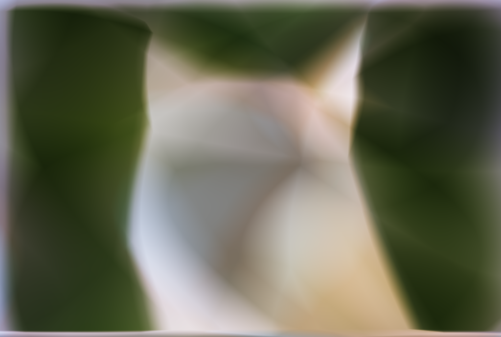
Shown below are two example images used during the calibration process.

Part 0.2: Capturing a 3D Object Scan

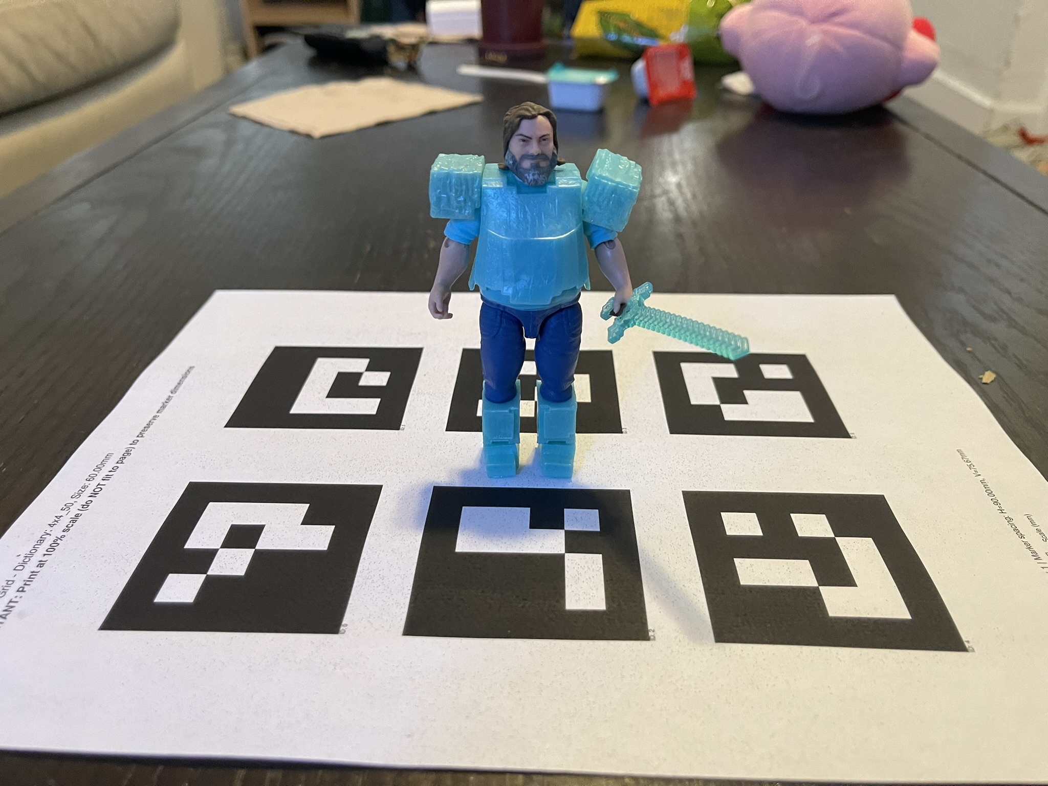
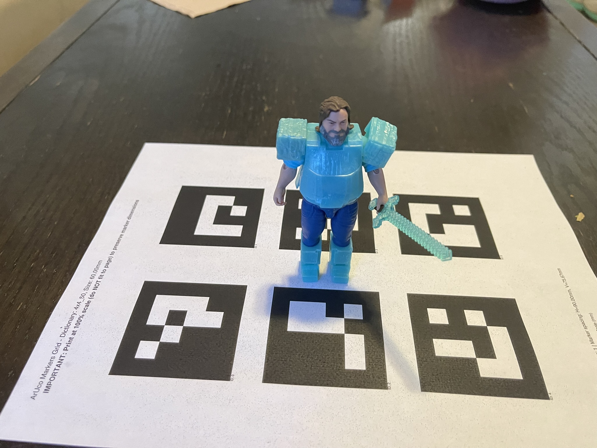
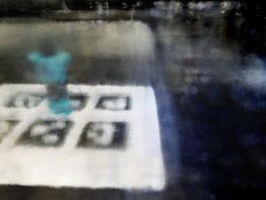
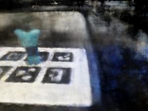
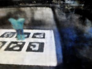
I captured approximately fifty images of the calibration tags with an object placed on top of them. The system allowed using either a single tag or the full set of tags from the calibration page. I chose to use all six tags because this guaranteed that at least one tag remained visible across all viewing angles.

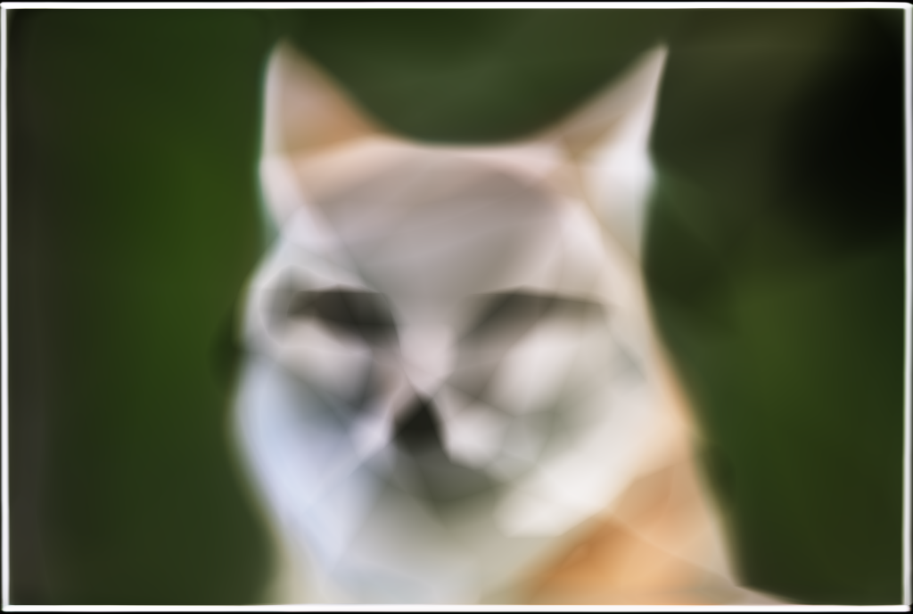
Shown below are two example images used for estimating the camera pose.

Part 0.3: Estimating Camera Pose

I used the intrinsic parameters of the camera to estimate the camera pose for each image of the object. This follows the classical perspective n point problem. Given a set of three dimensional points in world coordinates and their corresponding two dimensional projections in an image, the goal is to recover the camera extrinsic parameters, which consist of the rotation and translation. I used the function cv2.solvePnP() to obtain a rotation vector and a translation vector for each image. These outputs were then combined to form the camera to world transformation matrix (c2w).

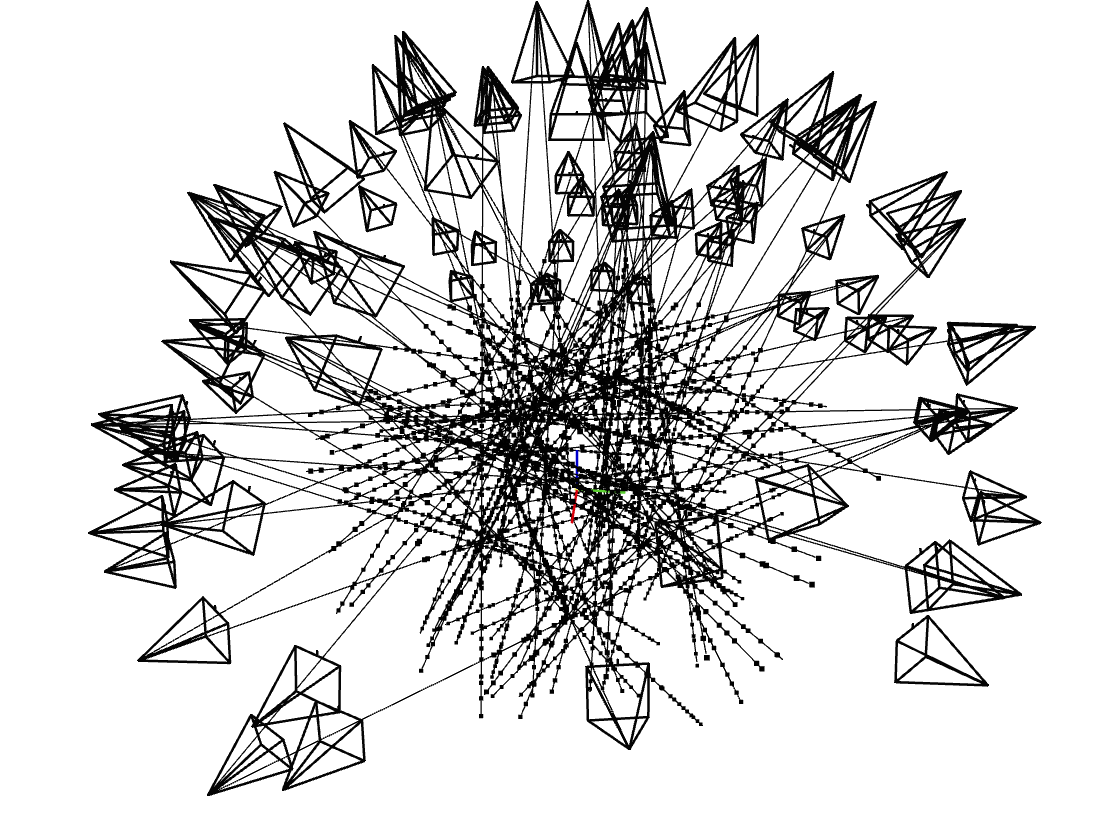
The pose estimation results were visualized by rendering the camera frustums in three dimensions using viser.

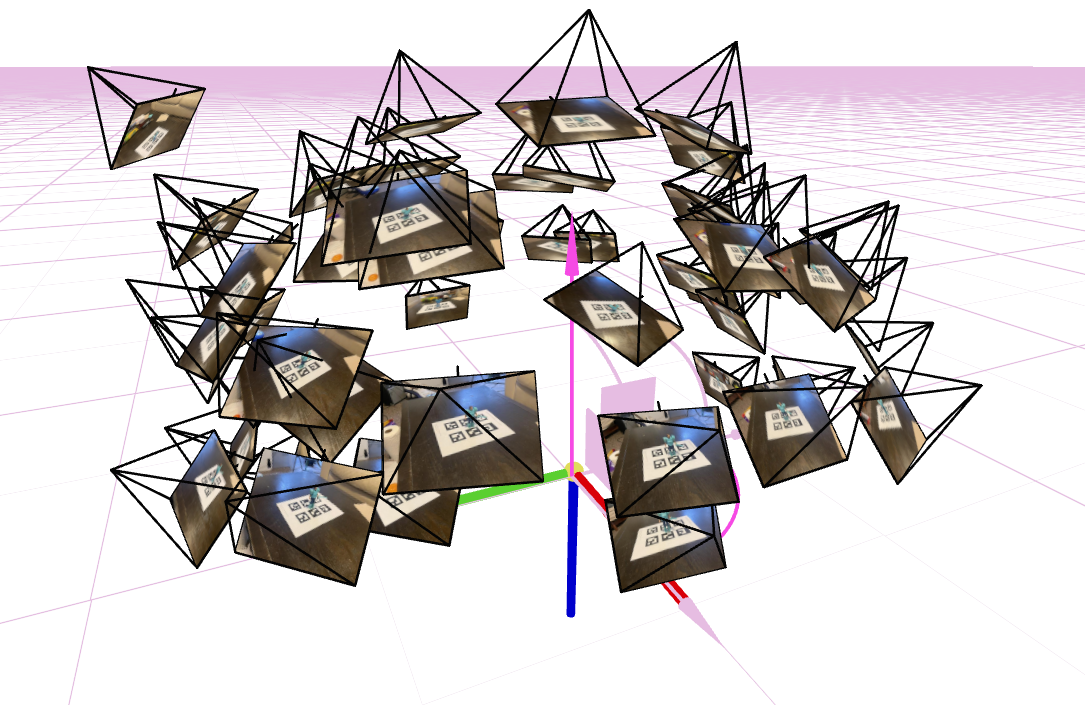
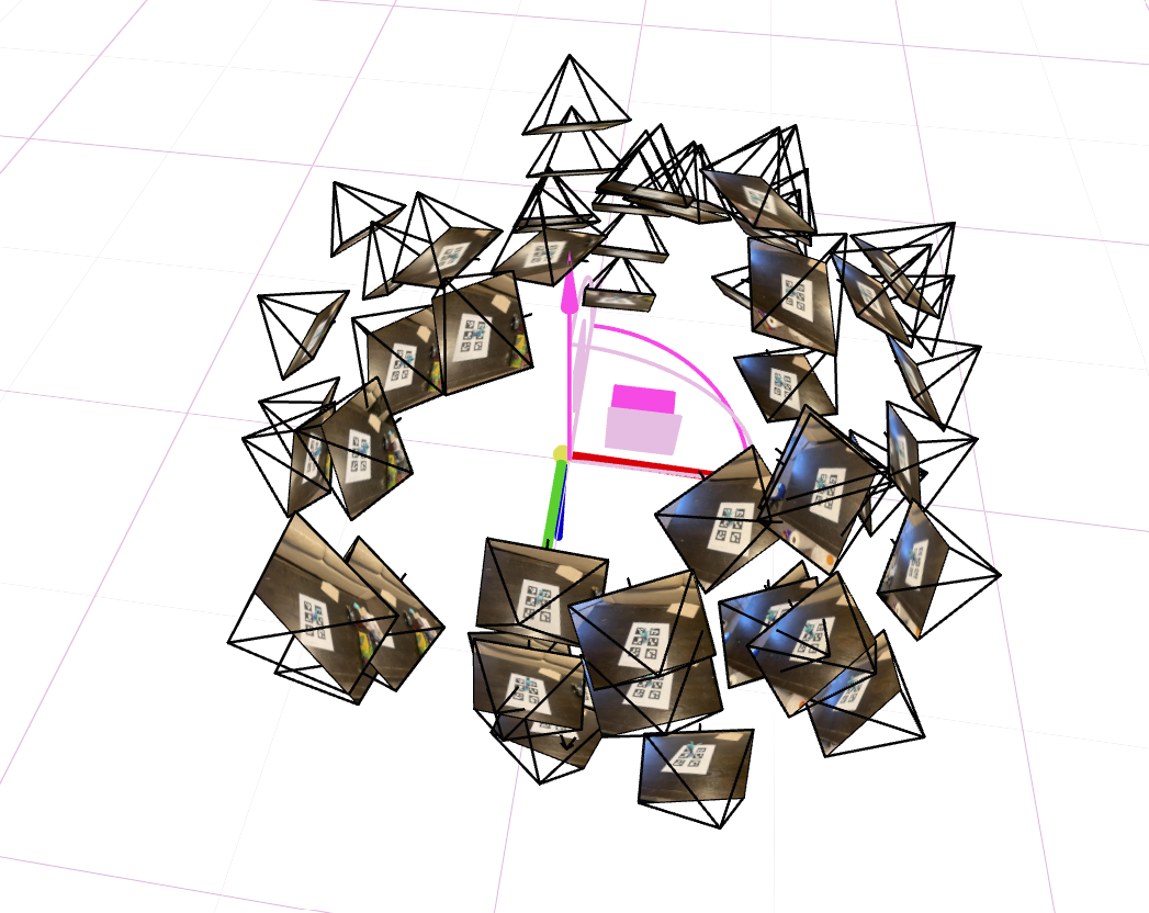
Part 0.4: Undistorting Images and Creating a Dataset

Using the camera intrinsics, the images were undistorted with cv2.undistort(), which removed lens distortion from the captures. This step is essential because NeRF assumes an ideal pinhole camera model without distortion.

A suitable maximum side length of 300 pixels was chosen for the images. This resolution kept the training process tractable while preserving as much detail as possible. All images were resized so that their longest side did not exceed this value.

The images and their corresponding extrinsic parameters were then divided into a training set and a validation set with 90 percent going to the training set. A test set was created by selecting one of the extrinsic translations as a reference point and generating a circular trajectory around the object, always pointing toward the origin. All resulting data was saved into a single npz file for use during training.

Part 1: Fit a Neural Field to a 2D Image

I trained a Neural Field that maps a pixel coordinate (u, v) to a predicted color (r, g, b). The goal in this section is to optimize the field so that it represents a single 2D image as accurately as possible.

Architecture

The model is composed of successive linear layers with ReLU activations, followed by a final sigmoid layer to ensure that the predicted color values lie in the range [0, 1]. Before entering the network, each input coordinate is transformed using a Sinusoidal Positional Encoding (PE), which expands its dimensionality. Positional encoding allows the model to represent high-frequency spatial detail that would otherwise be difficult for a standard MLP to capture.

In my implementation, the positional encoding used a max positional encoding frequency value (L) equal to 10, and each hidden layer had width 256. I also experimented with different hyperparameters, including reducing the hidden dimension to 16 and lowering the positional encoding level to 1.

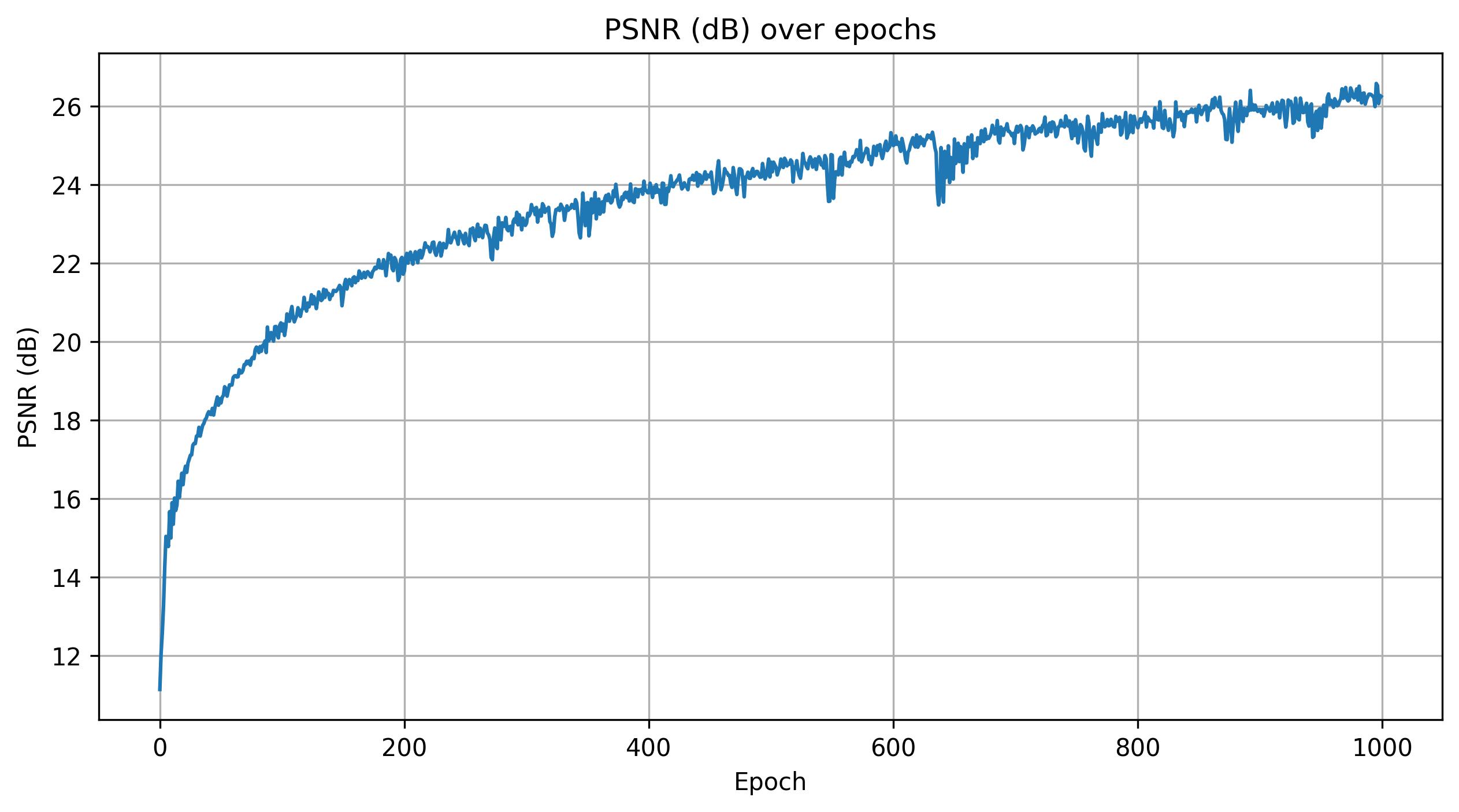
Training used an MSE loss and the Adam optimizer with a learning rate of 1e-2. The reconstruction quality was measured using peak signal to noise ratio (PSNR), which is defined by the equation \( PSNR = 10 \cdot \log_{10} \left( \frac{1}{MSE} \right) \). Image reconstruction was performed by passing every pixel coordinate of the image through the model and assembling the predicted RGB values back into an image.

Results

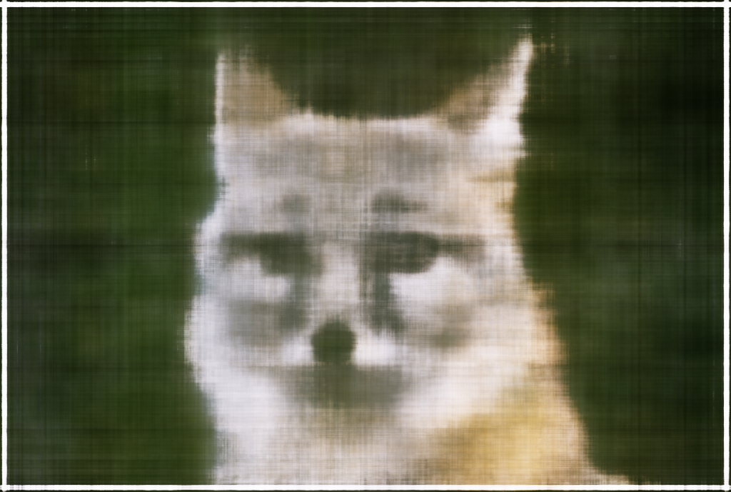
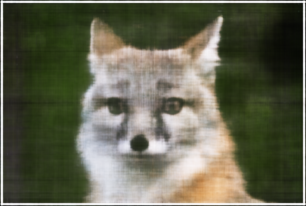
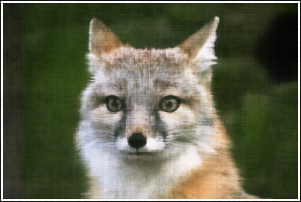
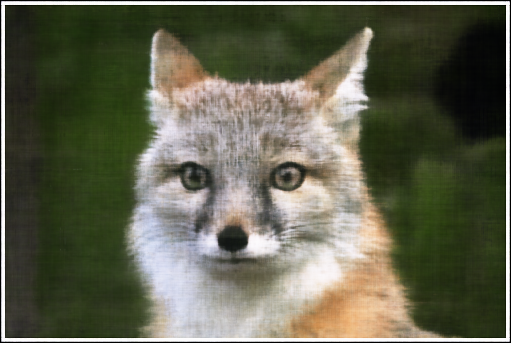
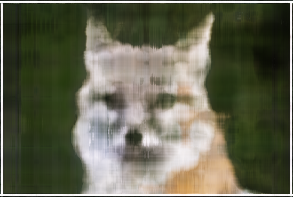
Shown below are the reconstructed images at various training iterations as the model attempts to fit the target image of a fox. These snapshots illustrate how the Neural Field progressively captures low-frequency structure before converging toward high-frequency detail.

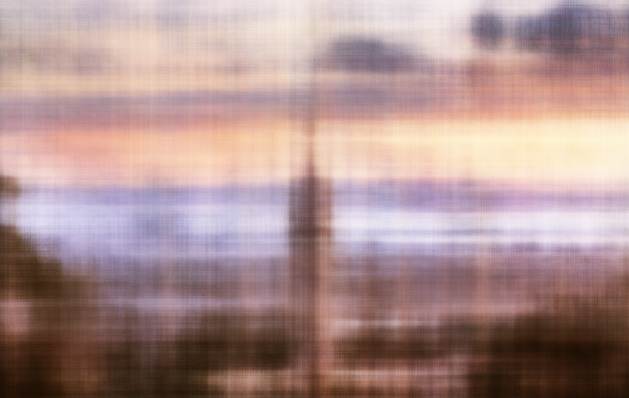
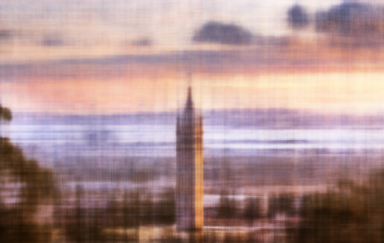
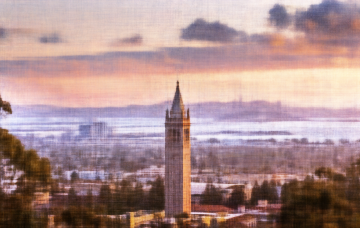
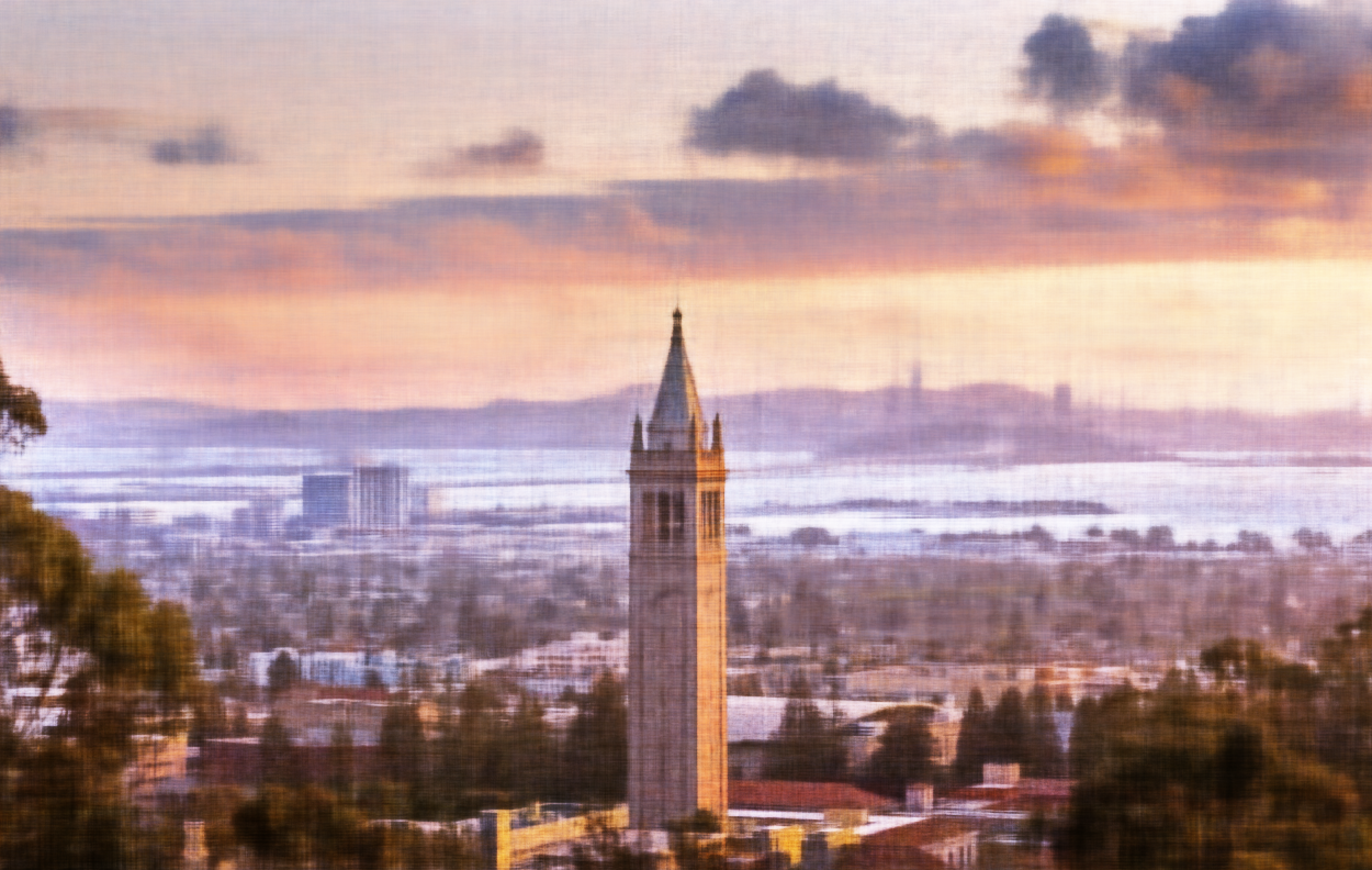
Shown below are the reconstructed images at various training iterations as the model fits a custom picture of Berkeley, along with the corresponding PSNR curve that tracks reconstruction quality over time.

Finally, the image below shows a 2×2 grid of reconstruction results generated by varying the maximum positional encoding frequency and the hidden layer width. The two values of L used were 1 and 10, and the two hidden layer widths were 16 and 256. Horizontally, the images vary by hidden layer width, while vertically they vary by maximum positional encoding frequency. Notice that the images on the bottom row lack high-frequency details.

Part 2: Fit a Neural Radiance Field from Multi-view Images

Part 2.1: Create Rays from Cameras

Here I implement three functions that support batching.

The first function, transform, takes a camera-to-world (c2w) transformation and a point in camera space (xc) and converts it to a point in world space (xw). This is done by multiplying xc by the rotation matrix from c2w and then adding the translation vector from c2w.

The second function, pixel_to_camera, takes a camera intrinsic matrix (K), a pixel coordinate (uv), and a depth (s) and transforms the pixel coordinate back into the camera coordinate system. The pixel is first converted to homogeneous coordinates, then multiplied by the inverse of K, and finally scaled by s.

The final function, pixel_to_ray, takes a camera intrinsic matrix (K), a camera-to-world transformation (c2w), and a pixel coordinate (uv) and converts it to a ray with an origin and normalized direction. The pixel is first converted to a camera coordinate at depth 1, then transformed to world coordinates. The ray origin is given by the translation component of c2w, and the ray direction is computed from the world coordinate and the ray origin.

Part 2.2: Sampling

Here I implement two additional functions that support batching.

The first function, sample_rays, takes a number N and randomly samples N rays from all of the rays in a RaysData object. It first computes a grid of all pixel coordinates in an image, which is then converted to rays using pixel_to_ray. These rays are stored as an attribute of the RaysData object. When sample_rays is called, it randomly selects N indices and returns the corresponding rays from this stored list.

The second function, sample_along_rays, takes ray origins, ray directions, and optional parameters such as perturb, near, and far. It discretizes each ray into 3D samples, uniformly spaced along the ray according to n_samples between near and far. To prevent overfitting from a fixed set of points, a small perturbation is added to each sample, drawn from a uniform distribution of (-width / 2, width / 2).

Part 2.3: Putting the Dataloading All Together

Here the RaysData object is implemented, which serves as a dataloader for the model. It is able to return ray origins, ray directions, and the corresponding pixel colors.

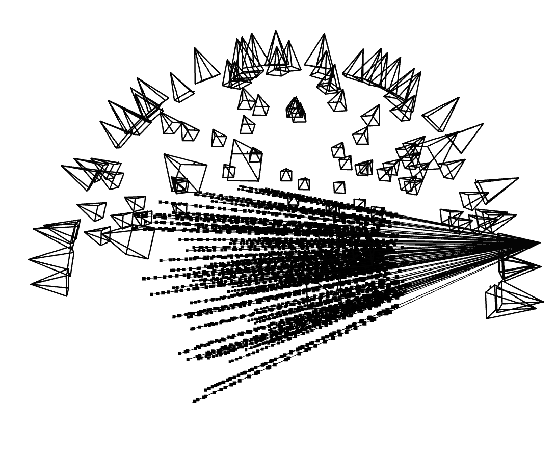
Shown below are the camera frustums with their rays visualized in Viser. On the left, each frustum emits a single ray, while on the right, one camera frustum emits one hundred randomly sampled rays. The dots along each ray represent the 3D sample points taken along that ray.

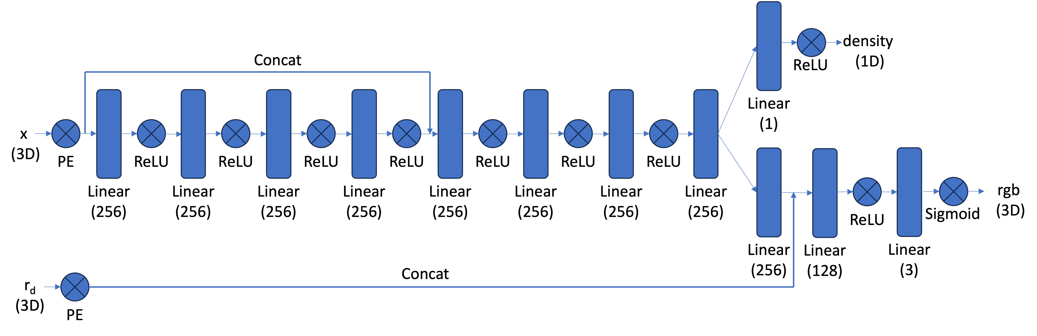
Part 2.4: Neural Radiance Field

Here the architecture of the NeRF model is constructed. This model is significantly more complex than its 2D counterpart because of the complexity of the scene it is modeling. Positional encodings are applied to both the world coordinates and the ray directions. The world coordinates are encoded with L = 10, while the ray directions use L = 4. All hidden layers have width 256.

The network uses a skip connection in the middle of the MLP, where the original input (after positional encoding) is concatenated back into the feature stream to help the model preserve high-frequency information. The network outputs two quantities through separate heads: one head predicts the density and the other predicts the color. I replaced the ReLU activation in the density head with a SoftPlus activation to improve training stability.

Part 2.5: Volume Rendering

The last function I implemented was volrend, which performs volumetric rendering to produce a final color for each ray. It takes the predicted density values (sigmas), RGB colors, and step sizes, and uses a discrete approximation of the NeRF volume rendering equation.

Each density value is converted into an alpha representing how much light is absorbed at that sample. These alphas are combined with per-sample transmittance to weight the contribution of each color along the ray. The final pixel color is obtained by accumulating these weighted colors, effectively simulating how light travels through a semi-transparent volume.

Results

Shown below is a rendering of the Lego scene from a viewpoint during different iterations of training, along with the corresponding PSNR curve, and a spherical rendering of the Lego model generated by orbiting the camera around the scene.

Part 2.6: Training With Your Own Data

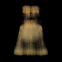
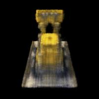
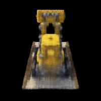
I decided to train on a Steve figurine from the Minecraft movie.

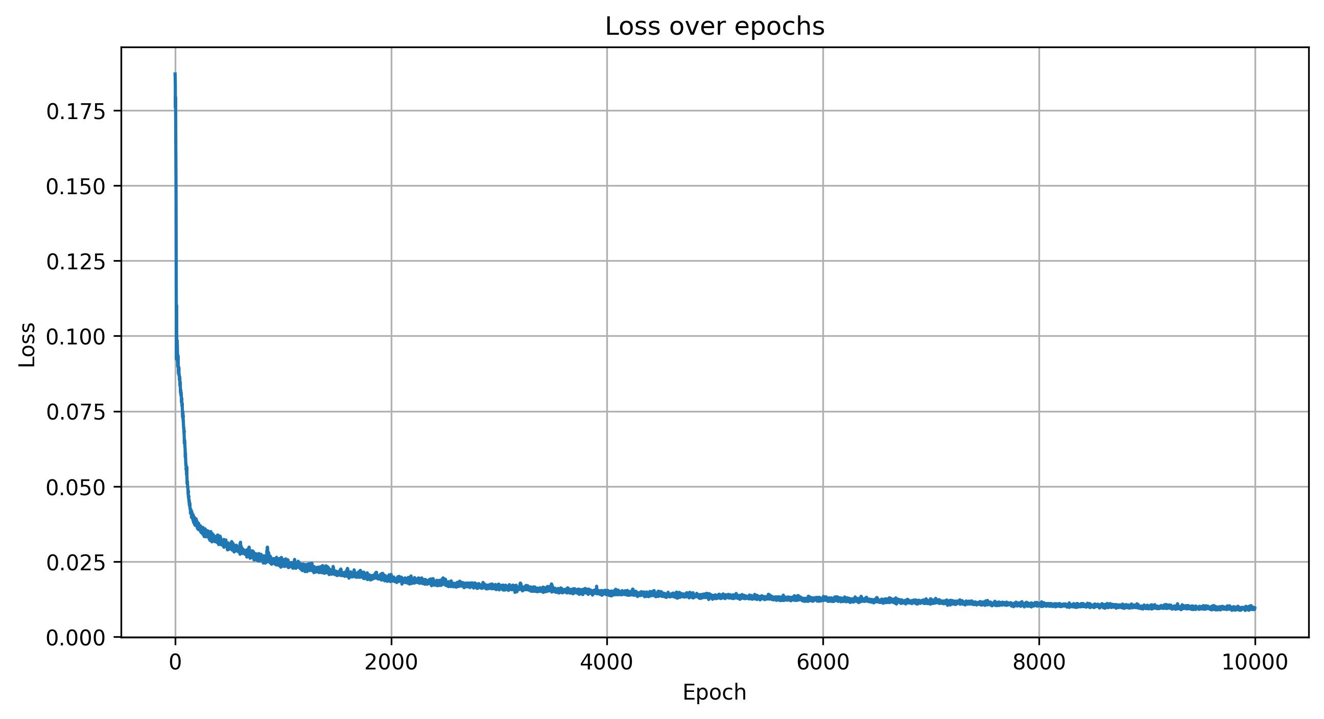
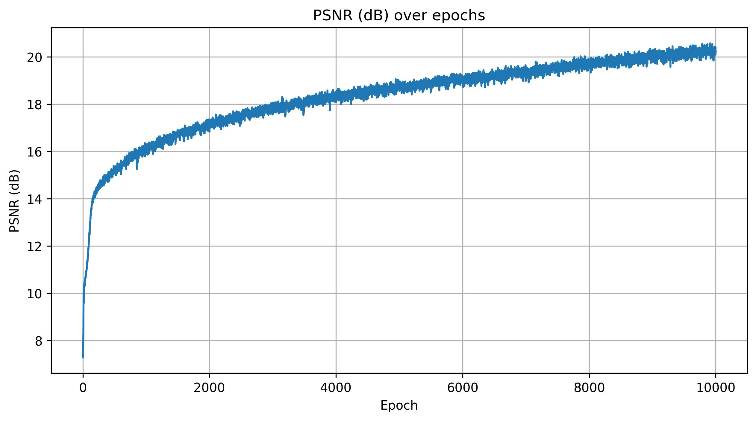
I used an MSE loss and trained the model with an AdamW optimizer with a learning rate of 5e-4 and a weight decay of 1e-5. The weight decay helped reduce overfitting and improved generalization. For sampling, I used near = 0.02 and far = 0.5 with 64 samples per ray, which I found to best cover the spatial extent of the object. I also increased the number of training epochs from 1000 to 10000 to allow the model to converge more fully on the scene.

Shown below is a rendering of a scene from a fixed viewpoint at different stages of training.

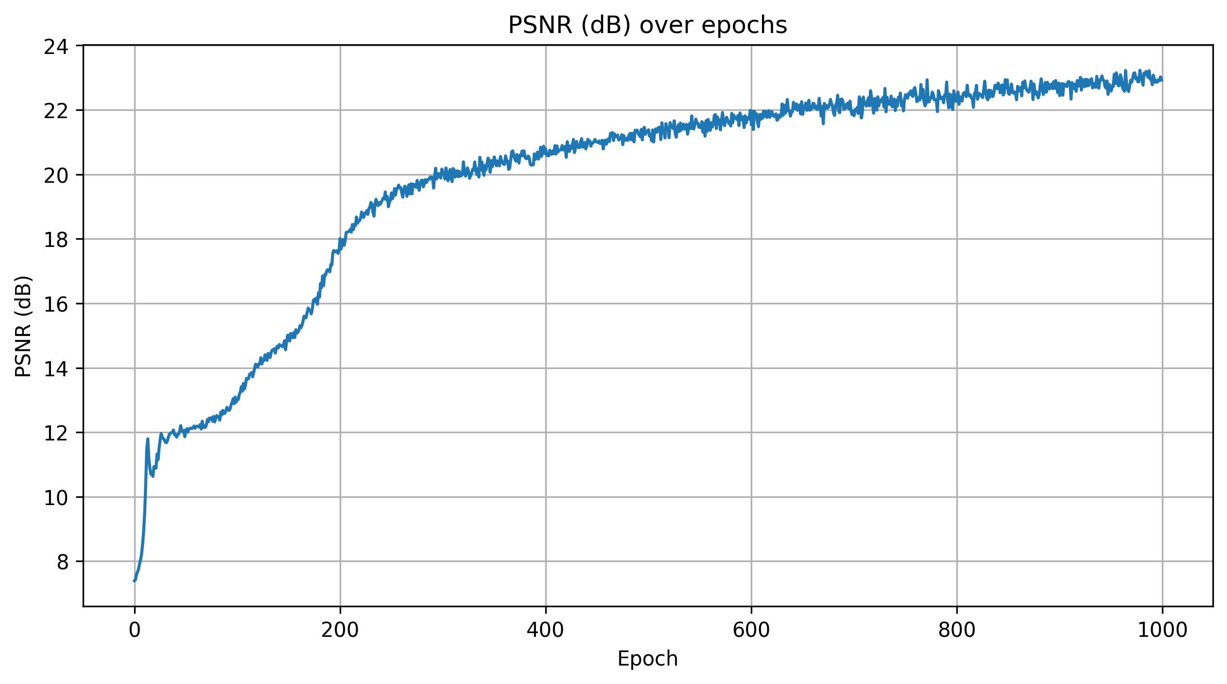
Shown below are the training loss and PSNR curves, along with a GIF of the camera circling around Steve.

Conclusion

Building the full NeRF system meant combining camera calibration, ray-based rendering, and a neural network that learns how a scene looks from different angles. The experiments showed how tools like positional encoding and sampling help the model learn detailed color and shape information from images alone. Training on my Steve figurine highlighted both the strengths of NeRF, such as generating accurate new views, and its challenges, including long training times and the need for good calibration. Overall, this project showed how a NeRF can use a set of photos to rebuild a 3D scene.