CS 180 Project 3: (Auto)stitching and Photo Mosaics

Introduction

This project explores the complete pipeline for image mosaicing, from manually selecting correspondence points to fully automatic feature-based stitching. The goal is to align and blend multiple overlapping images into seamless panoramas by estimating homographies that describe geometric transformations between views. In the first part, I implemented homography computation using least squares, image warping with interpolation, and image rectification. The second part focused on automation, using Harris corner detection with Adaptive Non-Maximal Suppression (ANMS), feature descriptor matching, and RANSAC for robust homography estimation. Together, these steps demonstrate how local feature analysis and projective geometry combine to achieve accurate and scalable image alignment.

Part 1: Image Warping and Mosaicing

Part 1.1: Shoot the Pictures

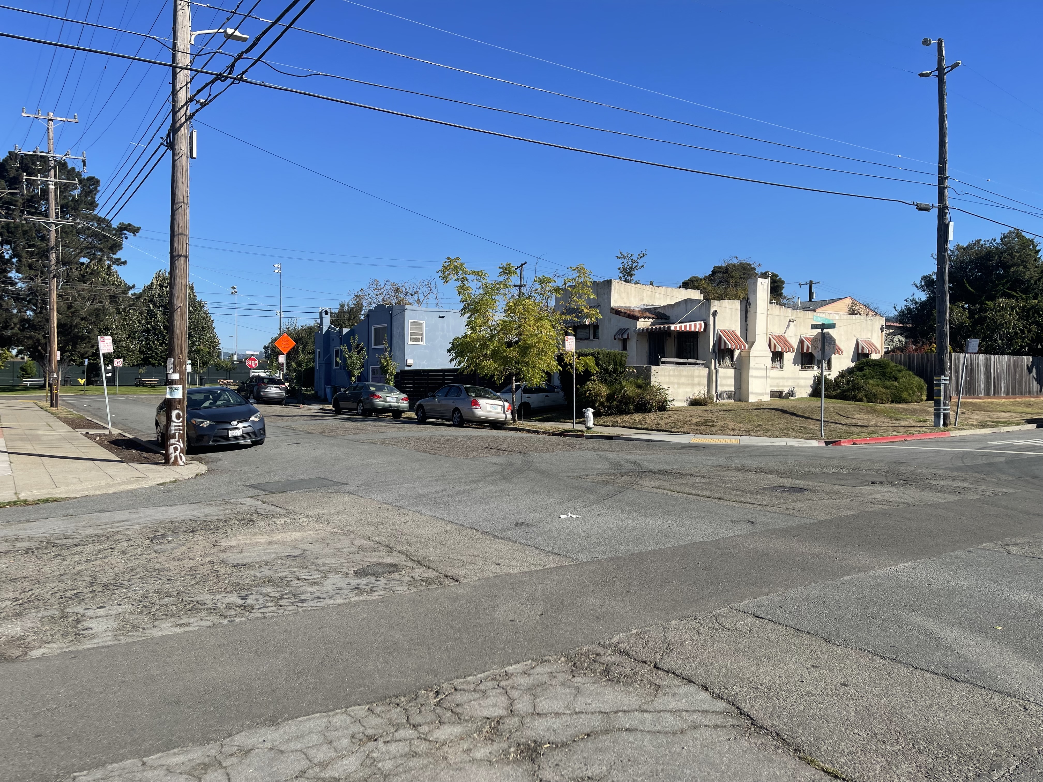
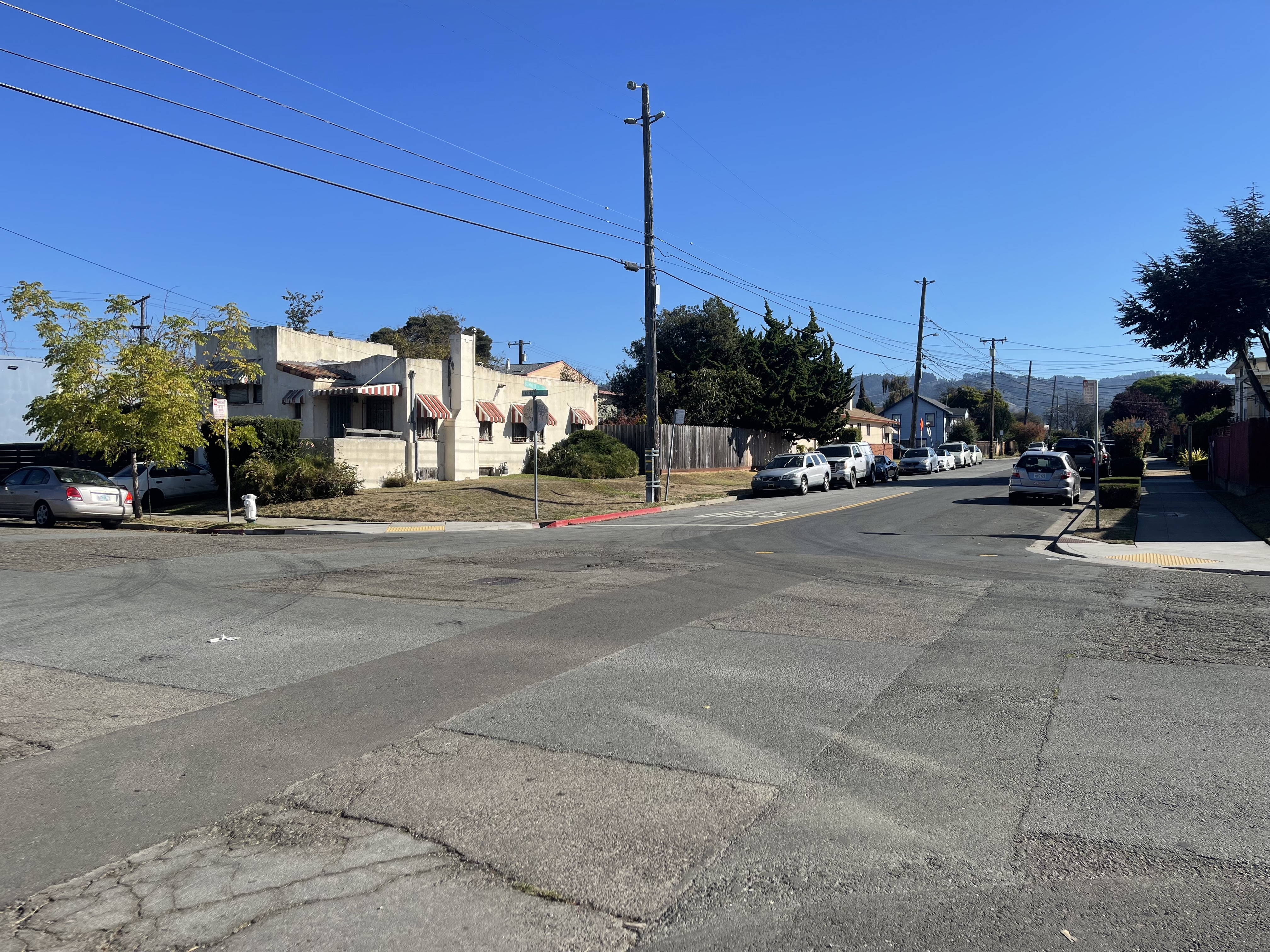
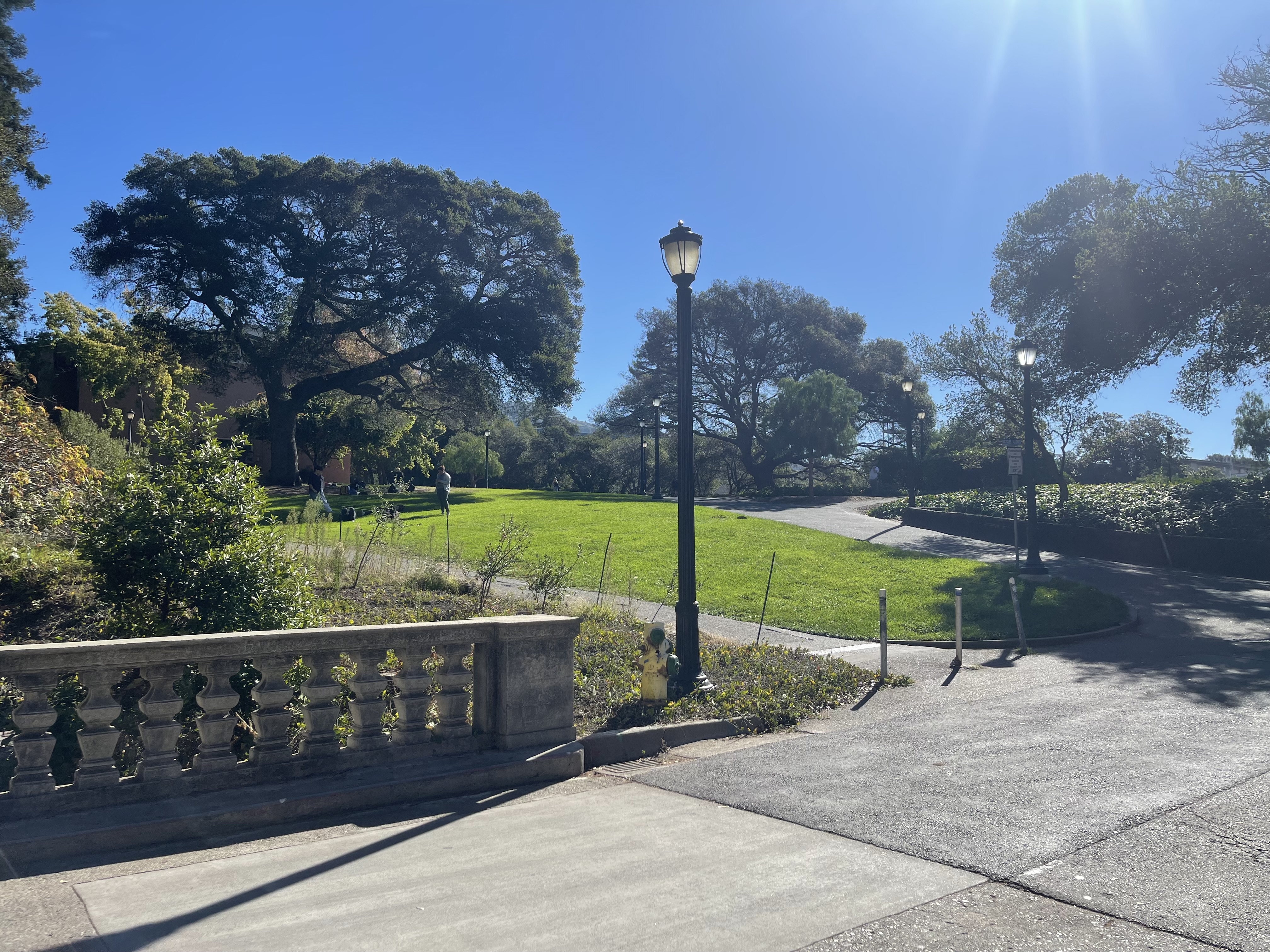
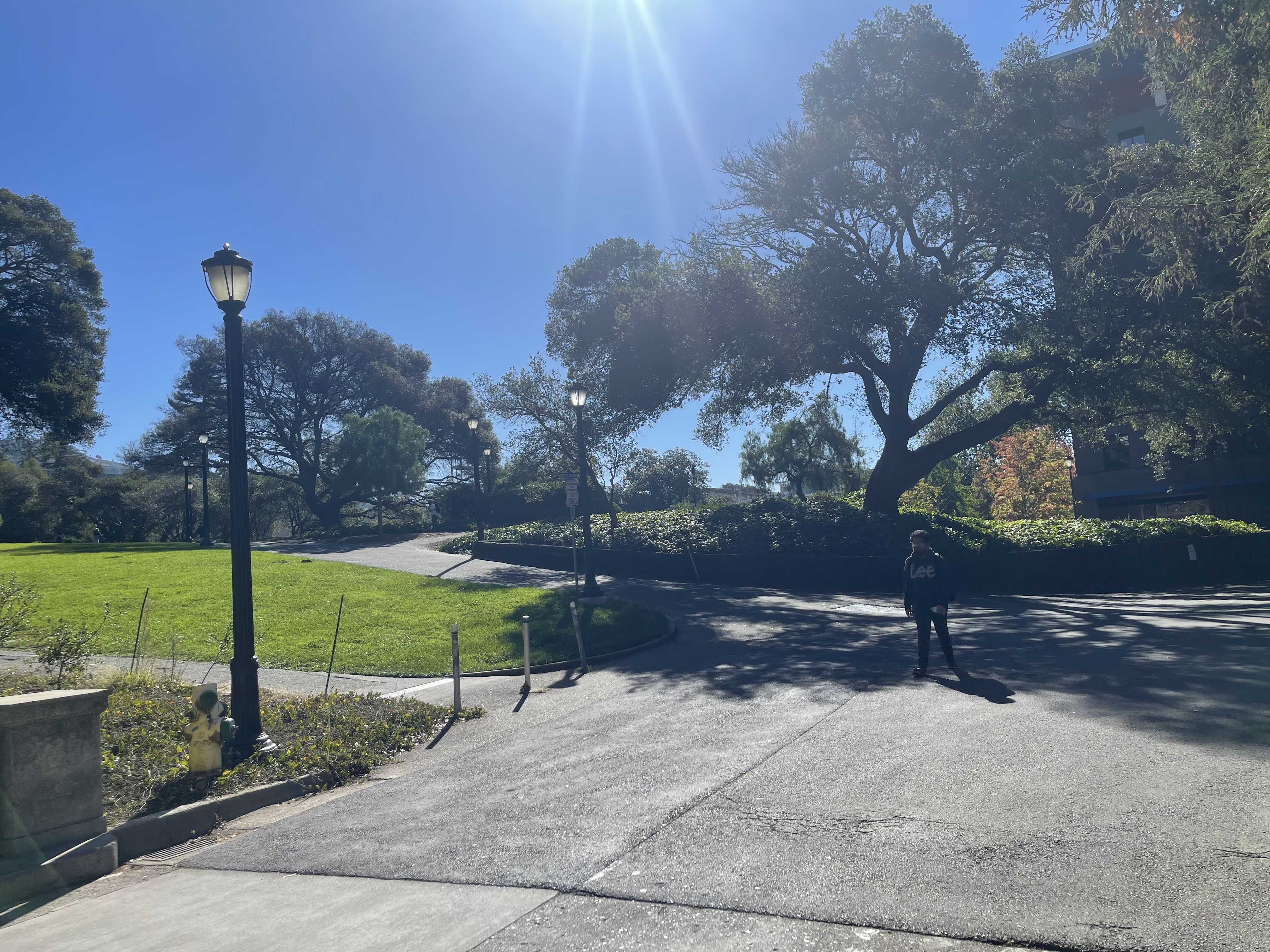
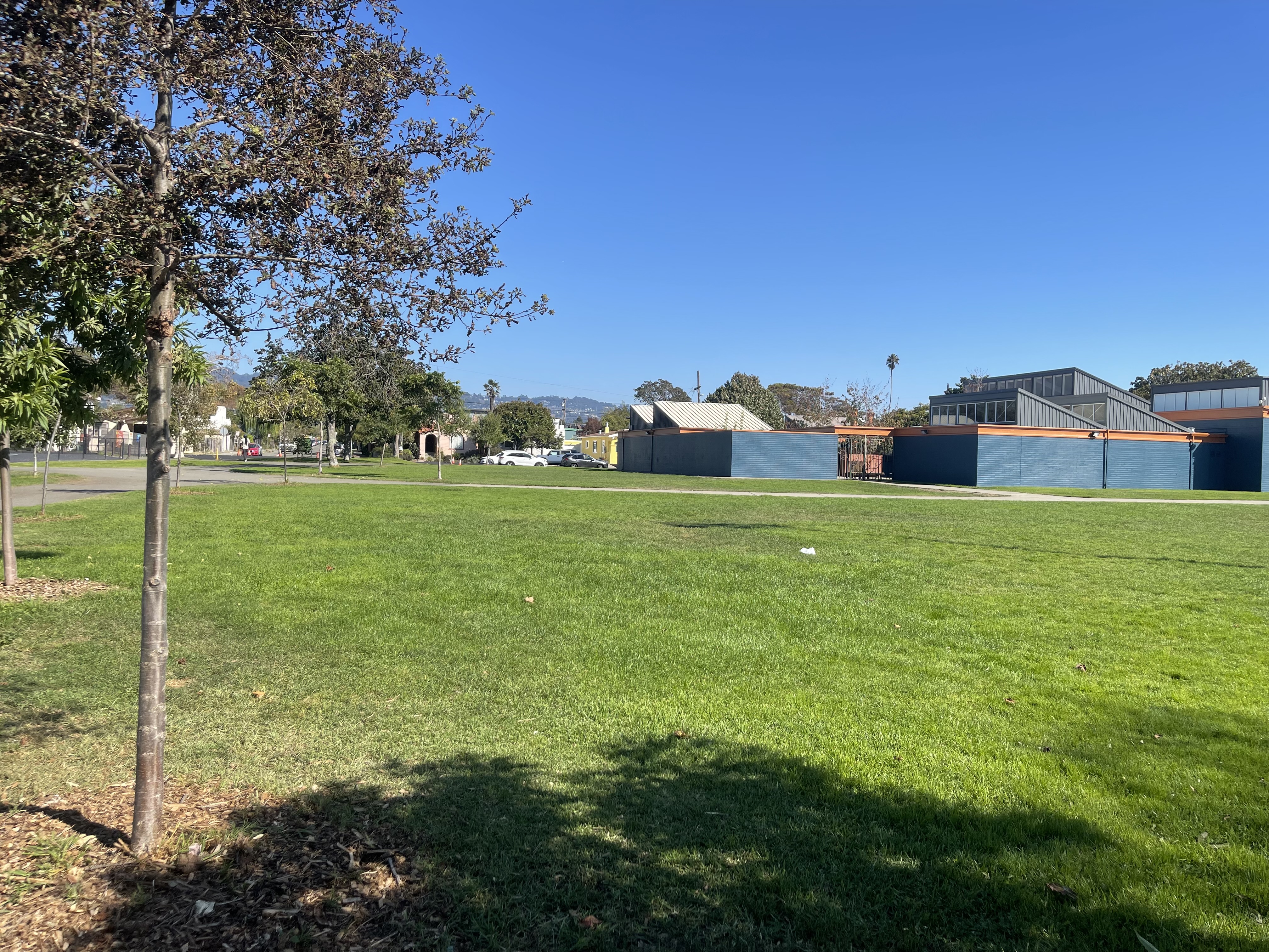
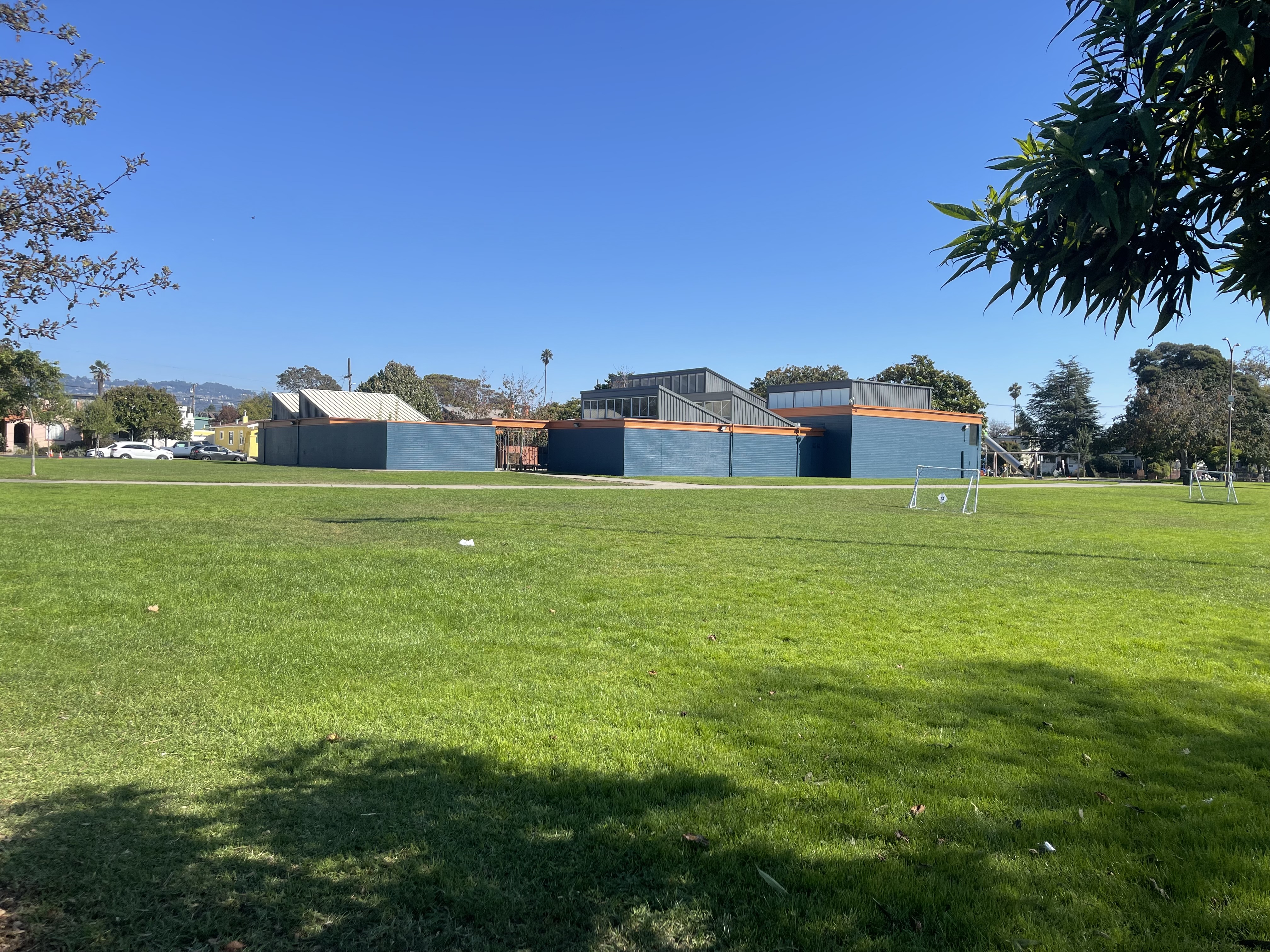
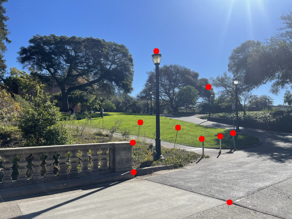
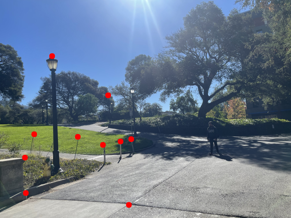
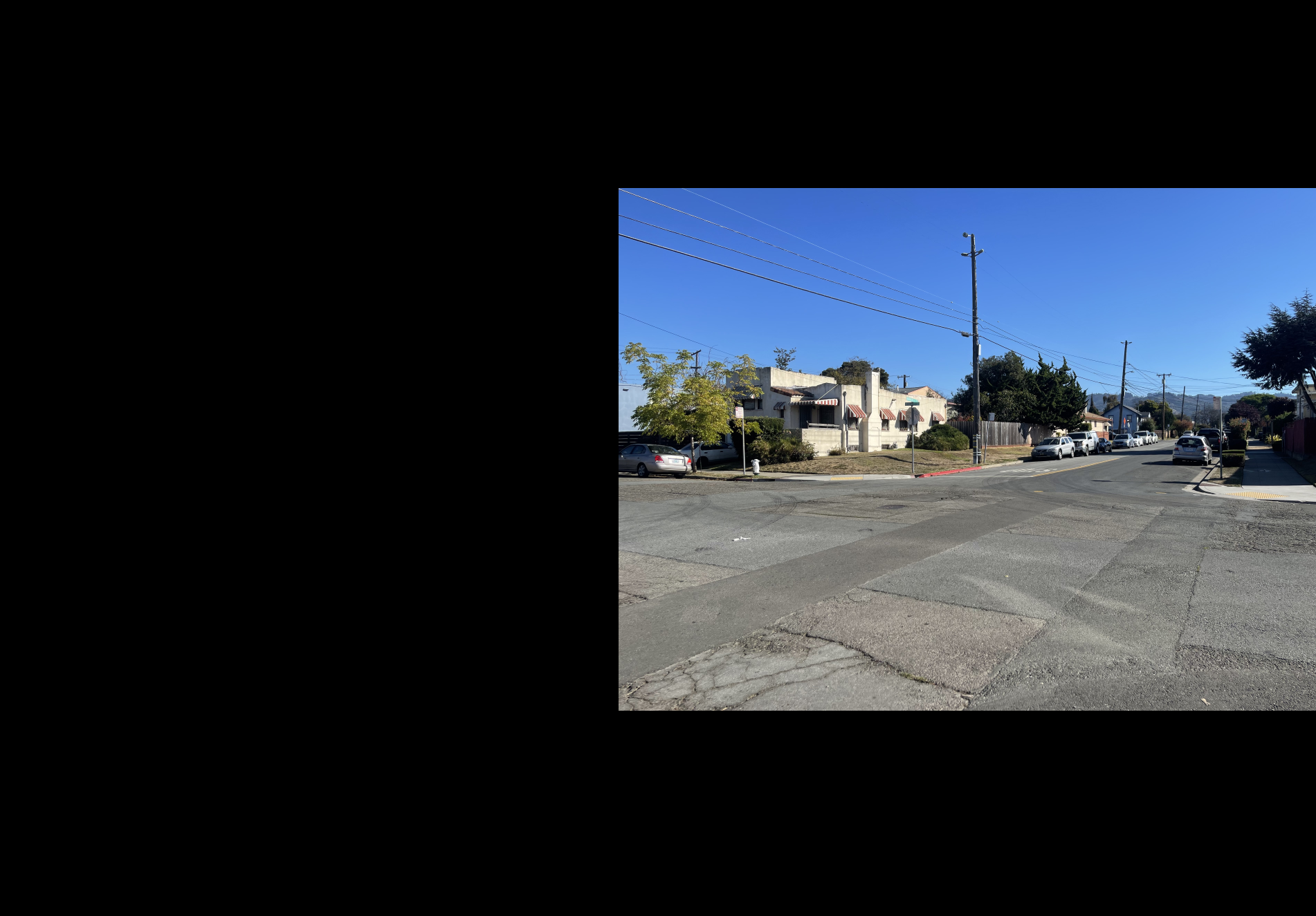
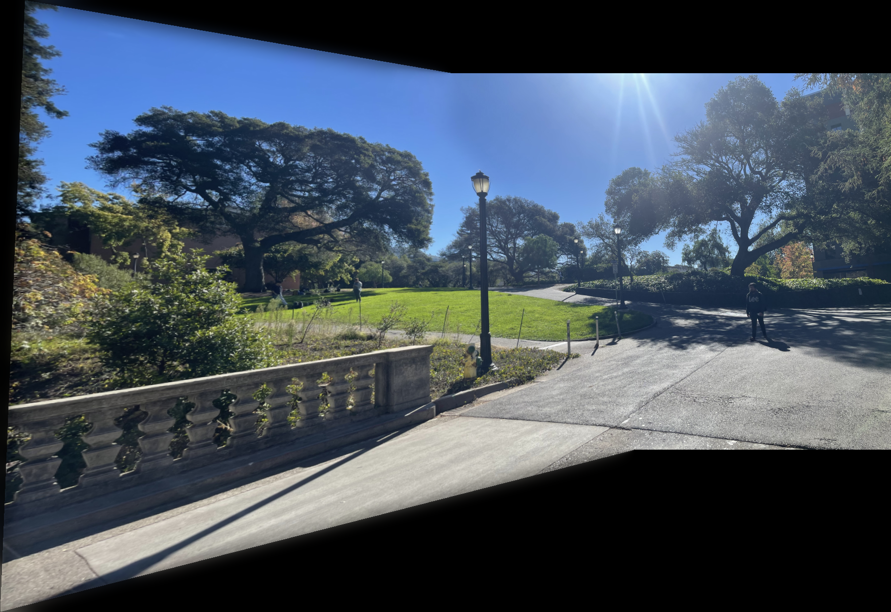
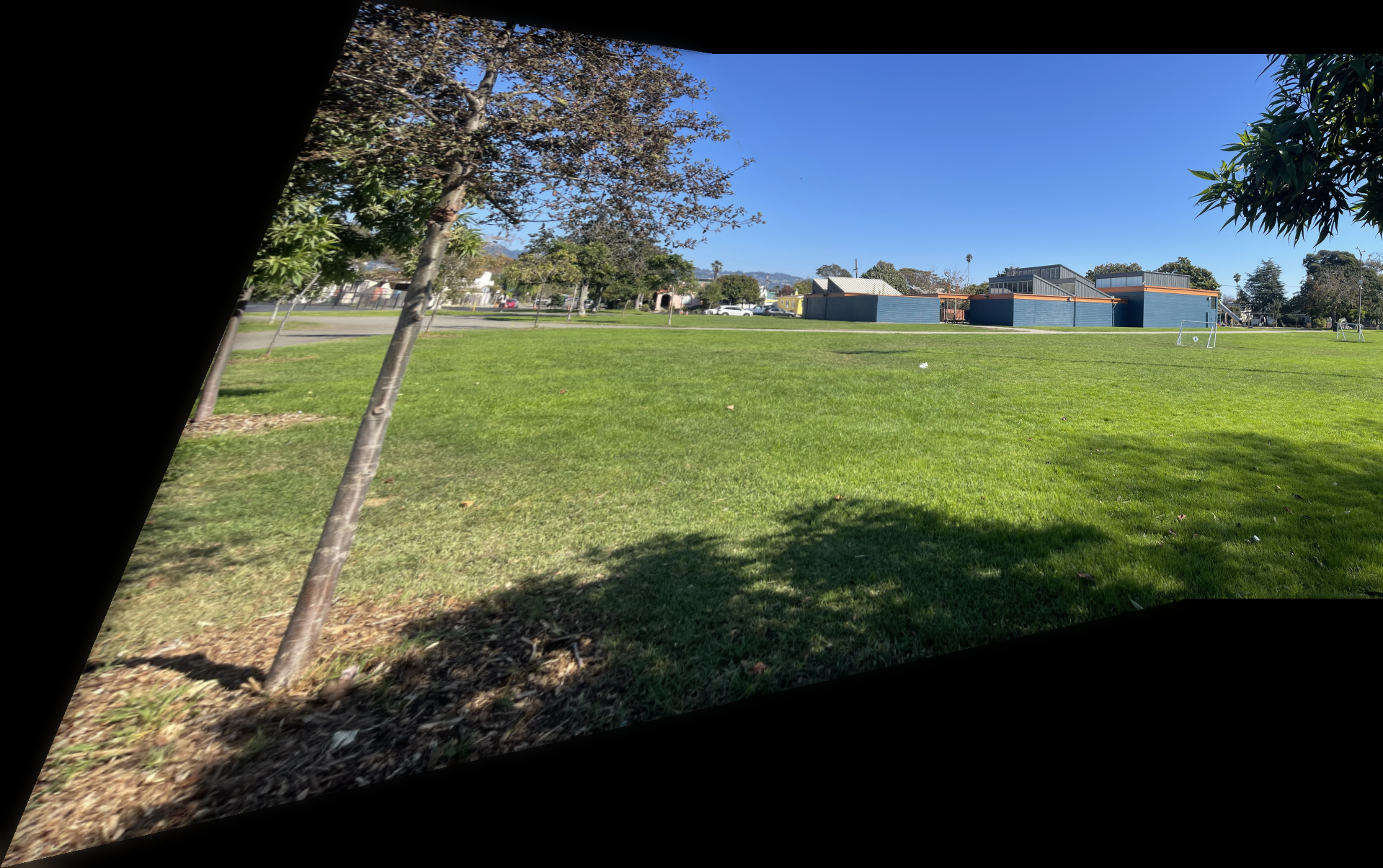
I captured pairs of photographs with projective transformations by keeping the camera's center of projection fixed and rotating it between shots. The three pairs below demonstrate this setup.

Part 1.2: Recover Homographies

Mathematical Background

Before I can align the images, I first need to recover the parameters of the transformation between each pair. This transformation is a homography, defined as \(p' = Hp\) where H is a \( 3 \times 3 \) matrix with 8 degrees of freedom. A homography can be estimated from a set of corresponding points \((p', p)\) across two images. At least four pairs of correspondences are required to solve for \( H \), though more points are typically used to reduce noise from hand selection or slight camera movement. A point \( [x, y, 1]^{\top} \) in image 1 is related to point \( [u, v, 1]^{\top} \) in image 2 by: \[ \lambda \begin{bmatrix} u \\ v \\ 1 \end{bmatrix} = H \begin{bmatrix} x \\ y \\ 1 \end{bmatrix} \] where \( \lambda \) is a scalar factor. The homography matrix can be expressed as: \[ H = \begin{bmatrix} h_{1} & h_{2} & h_{3} \\ h_{4} & h_{5} & h_{6} \\ h_{7} & h_{8} & 1 \end{bmatrix} \] To estimate \( H \), I rewrite the correspondences as an ordinary least squares (OLS) problem (\( Ah=b \)), where \( h = [h_{1}, h_{2}, h_{3}, h_{4}, h_{5}, h_{6}, h_{7}, h_{8}]^{\top} \), is the vectorized form of the matrix. Expanding the earlier equation gives: \[ \begin{bmatrix} \lambda u \\ \lambda v \\ \lambda \end{bmatrix} = \begin{bmatrix} h_{1} & h_{2} & h_{3} \\ h_{4} & h_{5} & h_{6} \\ h_{7} & h_{8} & 1 \end{bmatrix} \begin{bmatrix} x \\ y \\ 1 \end{bmatrix} \] Expanding this out and eliminating \( \lambda \) yields two equations: \[ h_{1}x + h_{2}y + h_{3} + h_{7}(-ux) + h_{8}(-uy) = u \] \[ h_{4}x + h_{5}y + h_{6} + h_{7}(-vx) + h_{8}(-vy) = v \] Stacking these equations for all point correspondences produces the linear system: \[ \begin{bmatrix} x_{1} & y_{1} & 1 & 0 & 0 & 0 & -u_{1}x_{1} & -u_{1}y_{1} \\ 0 & 0 & 0 & x_{1} & y_{1} & 1 & -v_{1}x_{1} & -v_{1}y_{1} \\ x_{2} & y_{2} & 1 & 0 & 0 & 0 & -u_{2}x_{2} & -u_{2}y_{2} \\ 0 & 0 & 0 & x_{2} & y_{2} & 1 & -v_{2}x_{2} & -v_{2}y_{2} \\ & & & & \vdots \end{bmatrix} \begin{bmatrix} h_{1} \\ h_{2} \\ h_{3} \\ h_{4} \\ h_{5} \\ h_{6} \\ h_{7} \\ h_{8} \end{bmatrix} = \begin{bmatrix} u_{1} \\ v_{1} \\ u_{2} \\ v_{2} \\ \vdots \end{bmatrix} \] Solving this least squares system yields \(h\), from which the homography matrix \( H \) is reconstructed.

Implementation

I selected correspondence points using matplotlib's ginput() and saved them to a text file to avoid reselecting them each time. The function that gathers these points returns a list of all (x,y) correspondences for each image. I implemented H = computeH(im1_pts, im2_pts), described below. To compute the homography, I initialized matrix \( A \) and vector \( b \) as empty arrays. For each pair of points in the correspondence list, I converted them into the OLS form shown earlier and appended the results as rows to \( A \) and \( b \). After processing all points, I used NumPy's linalg.lstsq() to solve for vector \( h \), which was then reshaped to reconstruct \( H \).

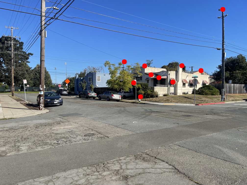
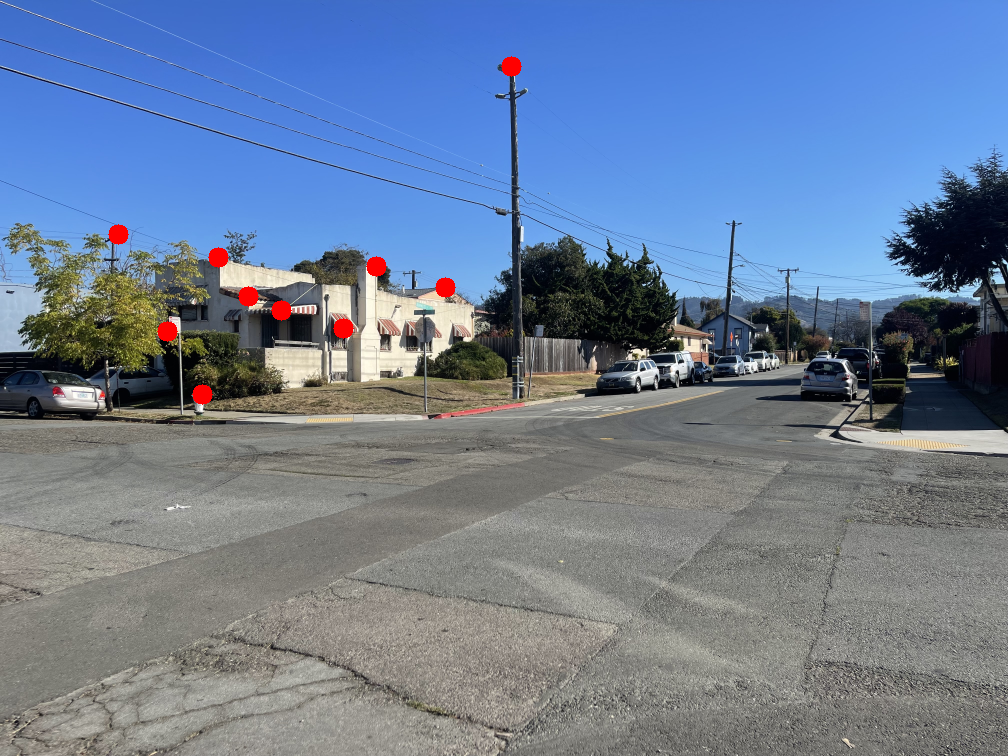
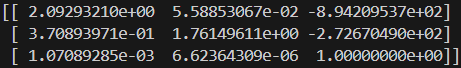
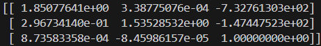
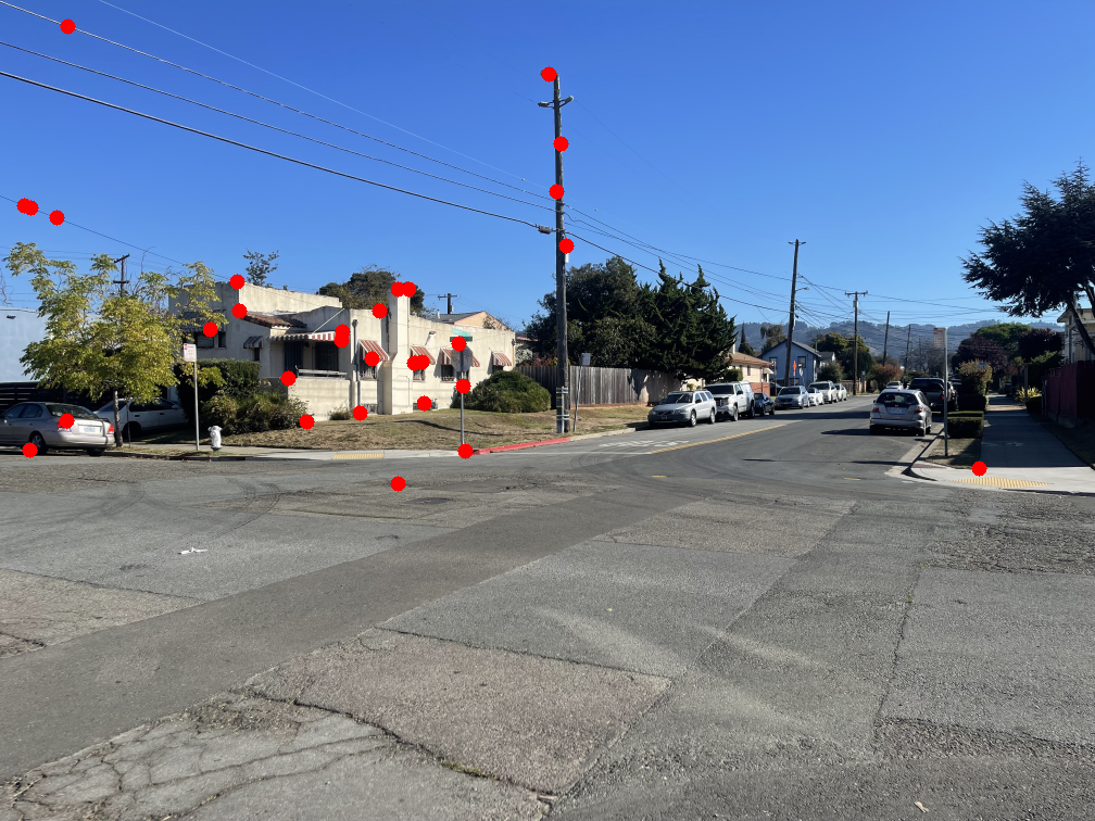
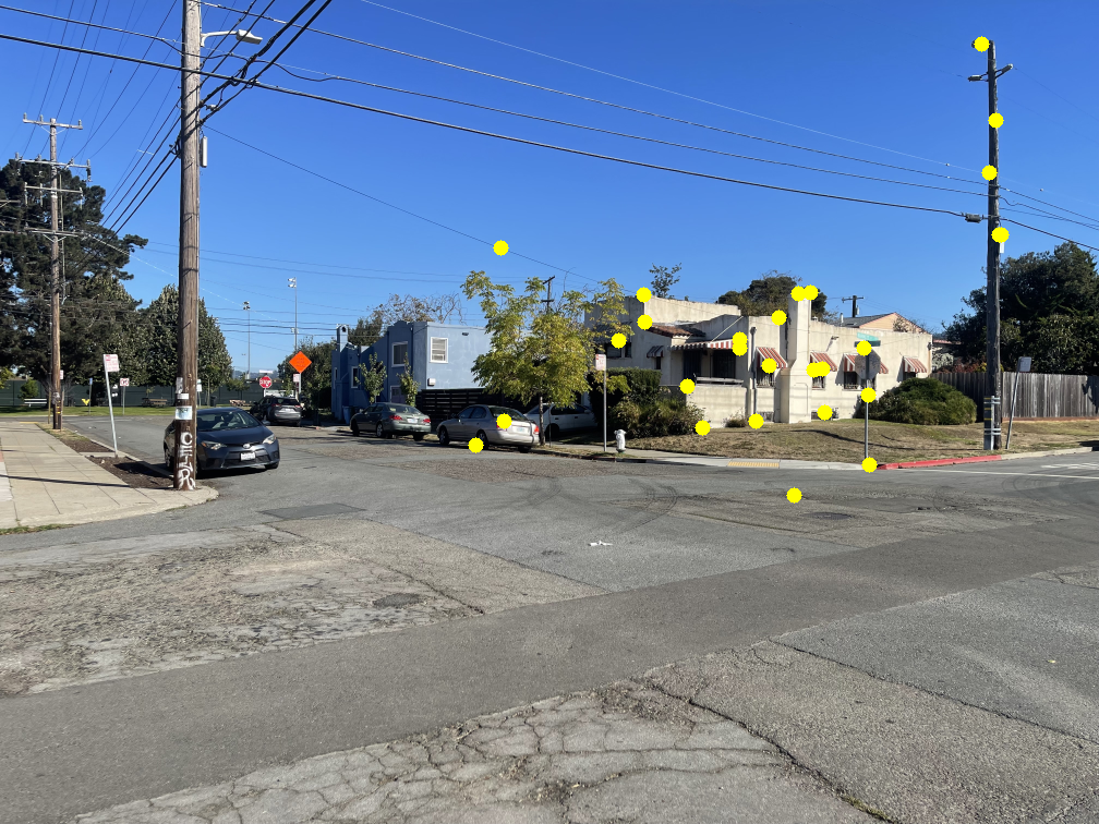
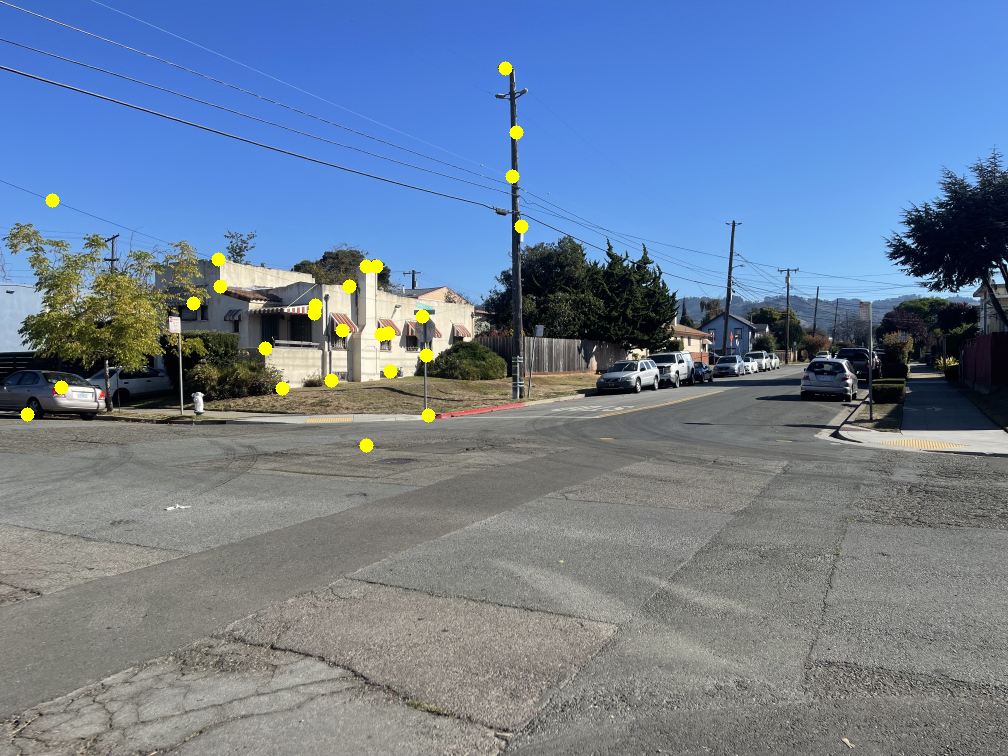
The images below show the manually selected correspondence points for two image pairs and the resulting homographies computed from them.

Part 1.3: Warp the Images

Warping

In this section, I implement image warping using inverse warping, where I iterate over pixels in the output image rather than the input. I define the origin (0,0) at the top-left corner of the first pixel and treat pixels as rays. This convention simplifies the process by avoiding corner cases and the need for extrapolation when mapping pixels.

The first step is to determine the bounding box, which defines the output dimensions. Even if the warped image does not occupy the entire space, the bounding box ensures that all transformed points fit within the output frame. I compute it by applying the forward transformation to the four corners of the source image, then finding the minimum and maximum x and y coordinates among these transformed points. The output width and height are the differences between these extrema. Because the transformation can produce negative coordinates, and negative indices would cause wrapping, I apply a translation to shift the image so that all coordinates are positive. This shift becomes important later when blending images.

The warping process begins the same way for both interpolation methods. After computing the bounding box and image shift, I initialize the warped image with an alpha channel set to zero and append an alpha channel of ones to the input image. This setup ensures that only pixels with valid mappings are visible in the output, while unmapped areas remain black. Next, I invert the homography matrix \( H \) since output pixels are determined by their corresponding positions in the source image through \( H^{-1} \).

I then iterate over each pixel in the output image. Each pixel's coordinates are first shifted using the values from get_bounding_box() to keep all pixels in frame. The coordinates are converted to homogeneous form, multiplied by \( H^{-1} \), and then converted back to Cartesian coordinates to locate the corresponding position in the original image. Because this position may not align with integer pixel coordinates, interpolation is required. Let this mapped position be called the "sample pixel". The two interpolation methods implemented are explained below:

• Nearest neighbor interpolation: The sample pixel's coordinates are rounded to the nearest integer, and the corresponding value is taken directly.


• Bilinear interpolation: The original pixel's coordinates are floored to find the lower-left corner of the surrounding pixel box, denoted \(I_{11}\). The other corners \(I_{12}\), \(I_{21}\), and \(I_{22}\) are found by adding one to the respective x and y indices. Let the sample pixel be at \((x, y)\), and the pixels \(I_{ij}\) be at \((x_i, y_j)\). Two horizontal interpolations are computed as \(f(x, y_j) = (x_2 - x)I_{1j} + (x - x_1)I_{2j}\) for \(j = 1, 2\). A final vertical interpolation between these results gives the pixel's intensity: \( f(x, y) = (y_2 - y)f(x, y_1) + (y - y_1)f(x, y_2) \). This produces a smooth approximation of the pixel value based on its neighbors.

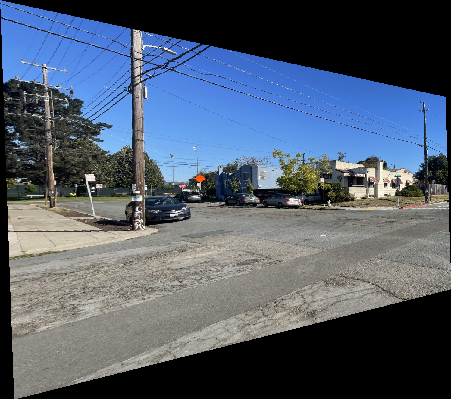
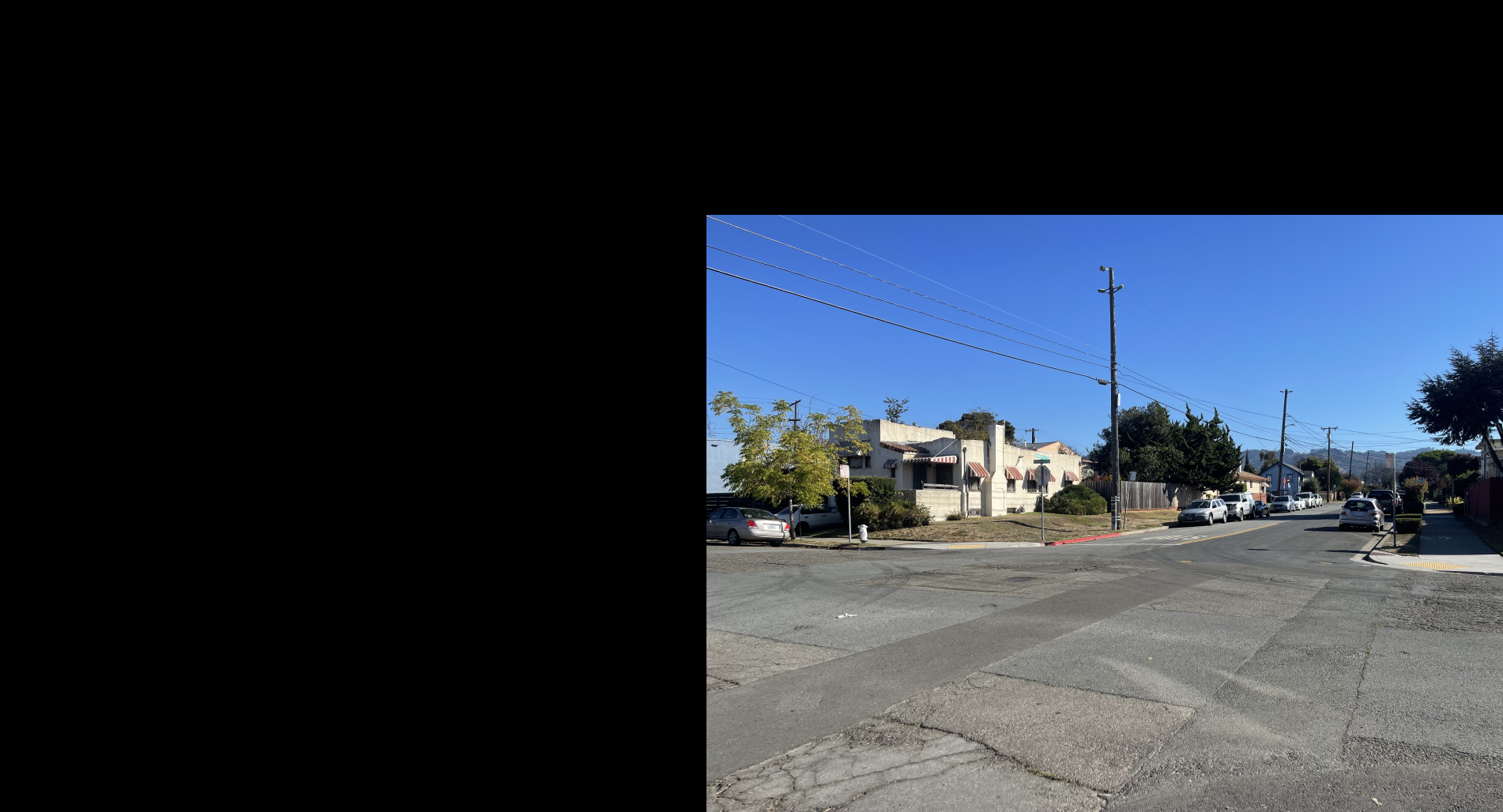
The results below show the warped versions of the “Left Image of Intersection” using nearest neighbor and bilinear interpolation. The difference is subtle, but the bilinear result appears smoother and less jagged. This is expected since bilinear interpolation computes each pixel as a weighted average of its neighbors, while nearest neighbor simply selects the closest pixel value. I also observed that the bilinear method runs slightly slower than nearest neighbor due to the additional computations involved.

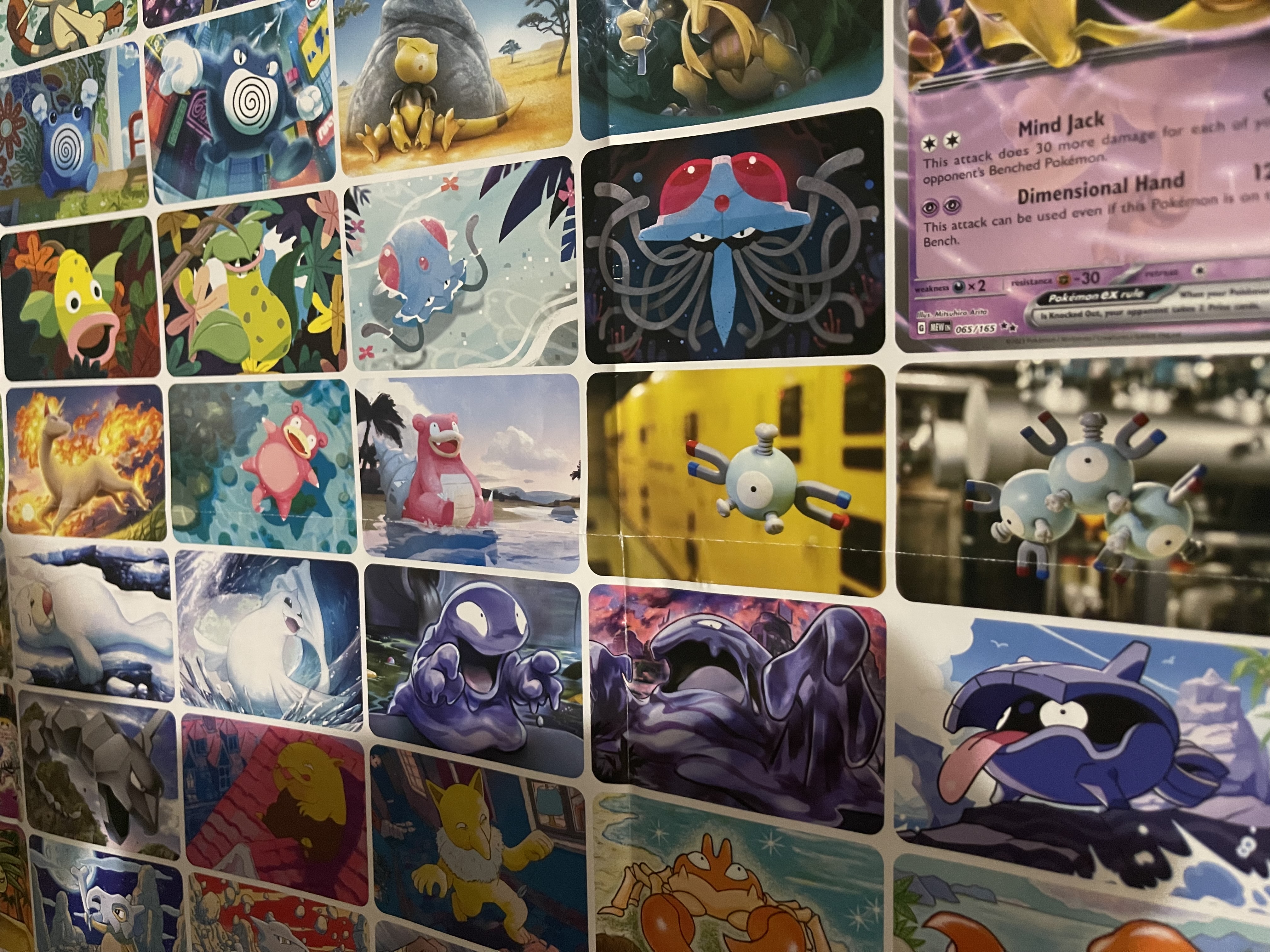
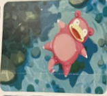
Rectification

Rectification involves taking an image of a known rectangular object captured from an angle and transforming it so the object appears rectangular rather than distorted. This is done by selecting four correspondence points on the image that match the four corners of the rectangle, then computing a homography using four reference points defined as \( [(0,0),(0,1),(1,1),(1,0)] \), starting from the top-left corner and moving clockwise. Because mapping directly to this unit square would result in a very small image, the points must be scaled. The scaling factor is estimated by measuring the actual size of the rectangle in the image, which is done by taking the maximum and minimum x and y coordinates among the four selected corners and subtracting the minimum values from the maximum values. This gives the approximate width and height of the rectangular region and produces the scaled reference points \( [(0,0),(0,h),(w,h),(w,0)] \).

Once the homography between these scaled points and the image correspondences is computed, warping can be performed. Since the goal is to align the image corners with the corners of the output frame, no displacement is applied when generating the output pixels. As a result, some regions outside the rectangular object are not mapped to the final image. After warping, the image is cropped automatically to the estimated width and height.

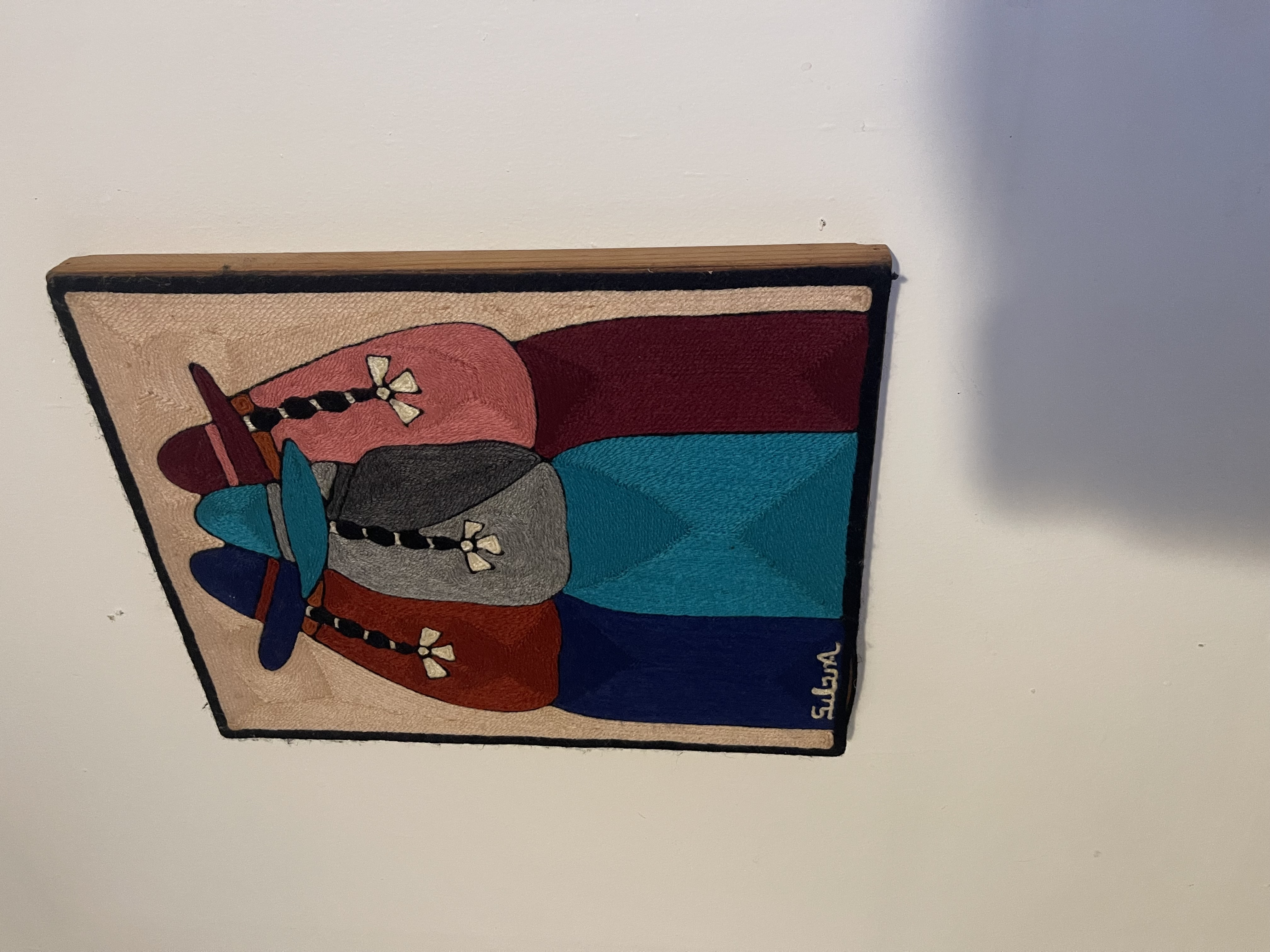
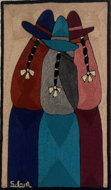
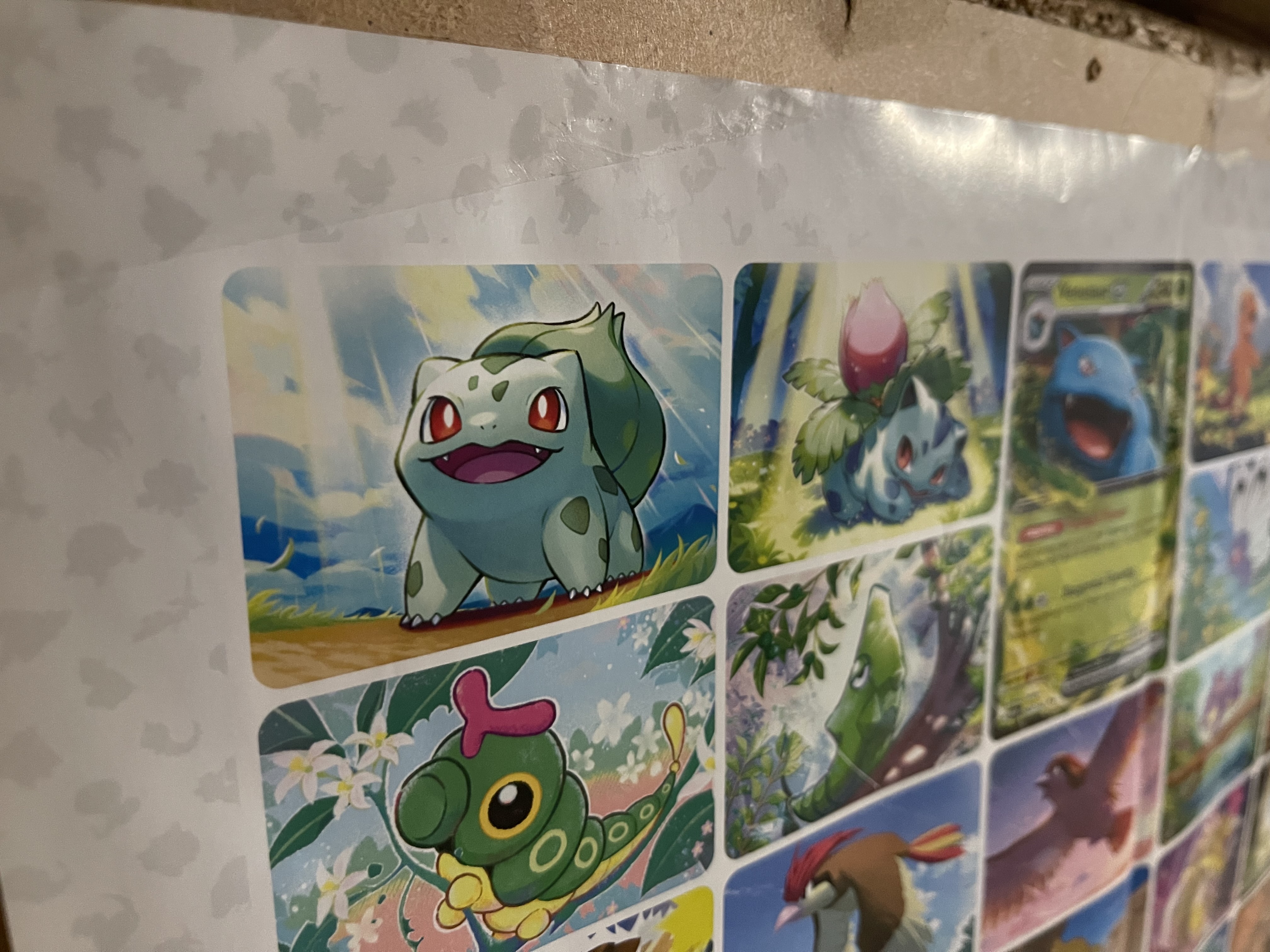
Shown below are examples of the resulting rectified images.

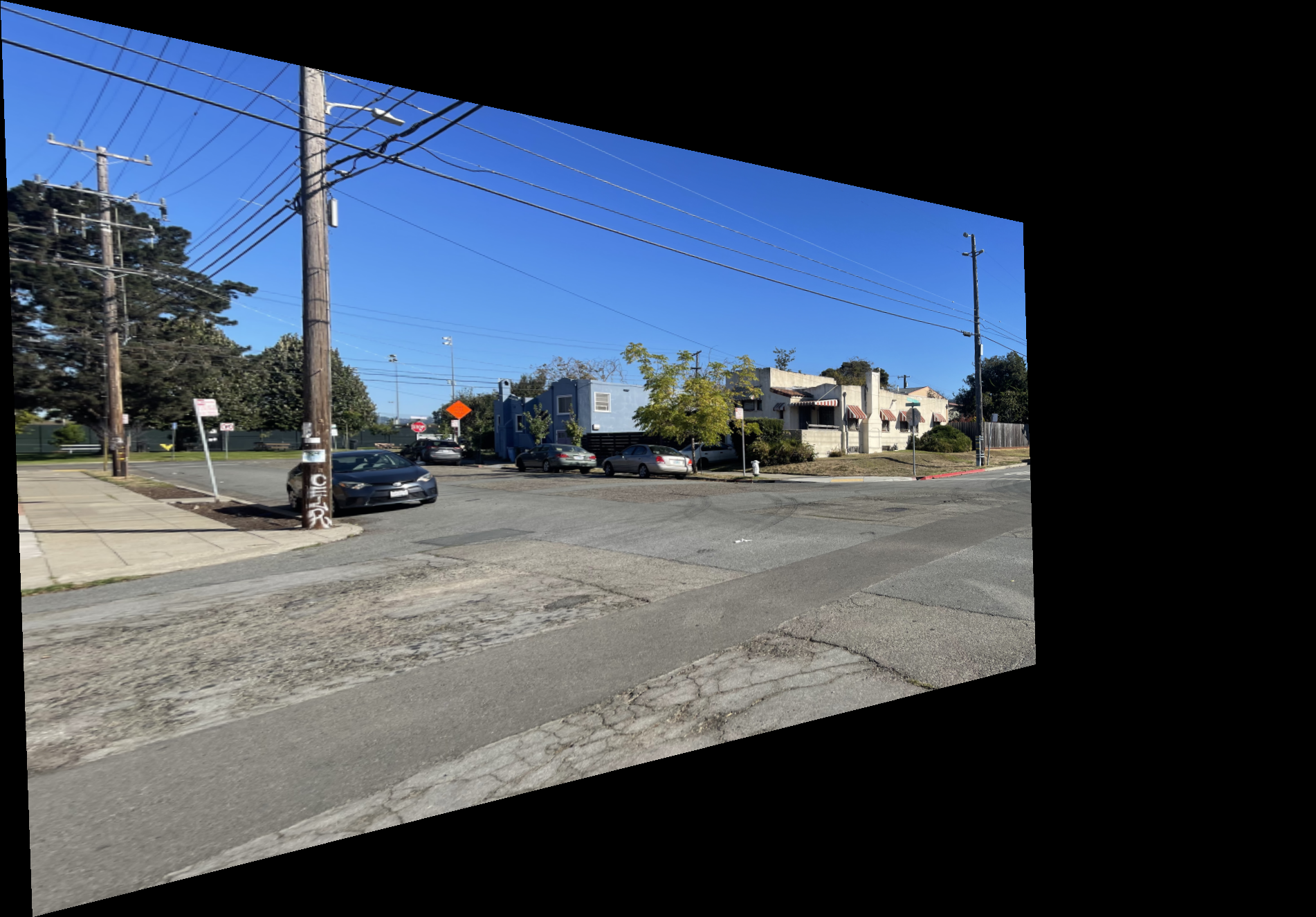
Part 1.4: Blend the Images into a Mosaic

In this section, I describe how I create a mosaic from two images related by a projective transform. For clarity, image1 refers to the image being warped, and image2 is the reference image. Using the functions defined earlier, I first compute a homography and warp image1 into the coordinate space of image2. Because this transformation can produce negative coordinates, the resulting image must be shifted to keep all pixels within valid bounds. If both images were combined without applying this shift to image2, they would not align properly. Thus, the same shift is applied to image2 to ensure alignment.

After alignment, both images are padded with zeros using np.pad() so they share the same dimensions and can be added together. Padding is applied only to the top and right edges to maintain their positions in coordinate space while simply extending the canvas size.

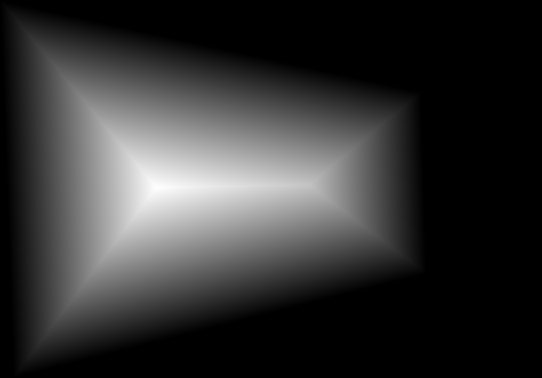
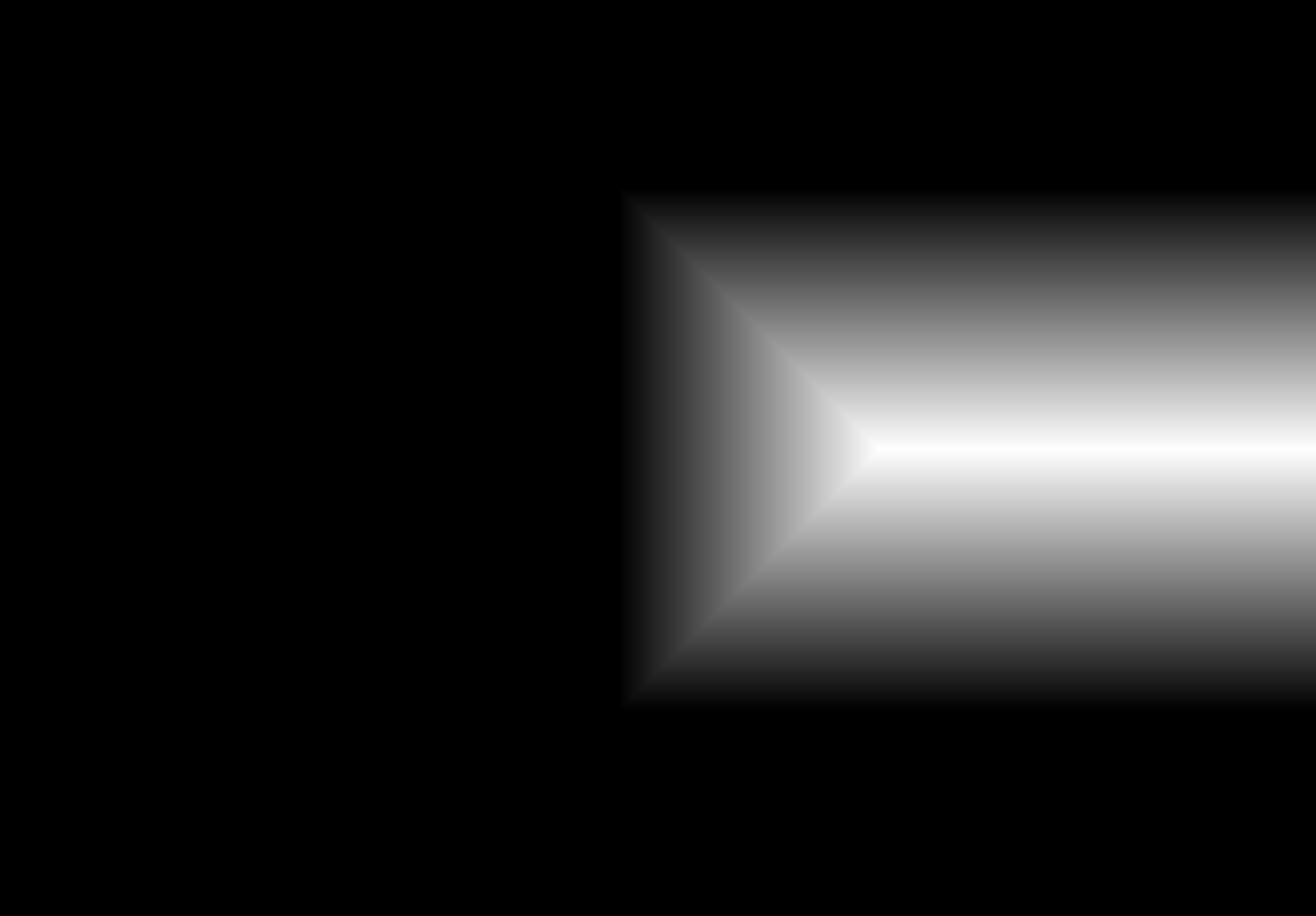
Once both images have matching dimensions, they can be blended to form a smooth mosaic. I use multiresolution blending with a specially constructed mask. The mask is generated by taking the alpha channels of each image, applying SciPy's ndimage.distance_transform_edt() to them, and comparing the results to form a binary mask (mask = logical(mask1 > mask2)). This mask defines which regions of each image contribute to the final blend and, together with the multiresolution blending, helps eliminate edge artifacts that would otherwise appear at the seams.

After the Laplacian pyramid layers are recombined, I clip all pixel values to the range [0, 1]. Clipping is used instead of min-max normalization since all intermediate operations are already normalized. Any small deviations are better corrected by trimming rather than stretching or compressing the values.

Shown below is the complete process for one image pair.

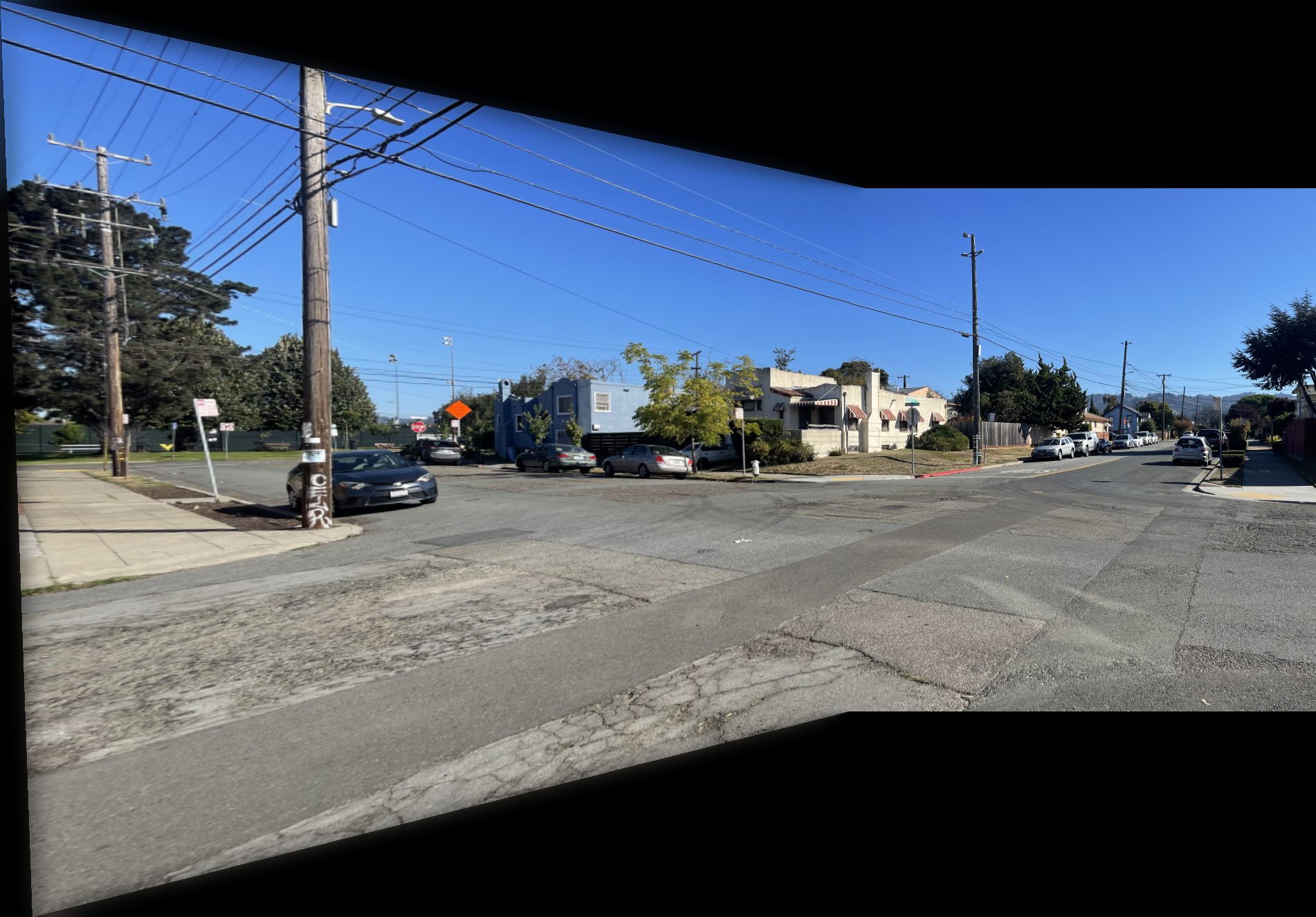
Shown below are additional examples of the resulting mosaics.

Part 2: Feature Matching for Autostitching

Selecting correspondence points manually can be tedious and time-consuming during mosaic creation. Fortunately, this process can be automated.

Part 2.1: Harris Corner Detection

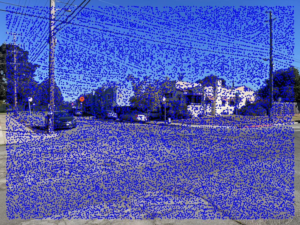
An effective way to locate points on an image is to detect corners. Here, I use Harris Corner Detection to identify interest points. The left image below shows Harris points overlaid on an example image.

As shown, there are many detected points. Using all of them would make the next steps in the autostitching process extremely slow. To address this, I apply Adaptive Non-Maximal Suppression (ANMS) to reduce the number of interest points while retaining the most informative ones. Simply choosing the strongest Harris points often results in poor spatial distribution, while selecting random ones risks losing the best features.

In ANMS, each point is assigned a suppression radius within which it remains the strongest by a factor of \( c = 0.9 \). To implement this, I iterate through all detected points. For each point \( x_i \), I examine its nearest neighbors starting from the closest and check whether \(f(x_i) > c \cdot f(x_j)\), where \( x_j \) is a neighboring point and \( f() \) returns the strength of the harris corner. If this condition fails, the radius \( r_i \) is set to the Euclidean distance between \( x_i \) and \( x_j \). After assigning radii to all points, I keep the k points with the largest suppression radii. These correspond to the most spatially distinct and significant corners, while the rest are discarded. For my implementation, I used \( k = 500 \). To efficiently find nearest neighbors, I used SciPy's cKDTree, which reduces search time from \( O(n^2) \) to roughly \( O(nlog(n)) \).

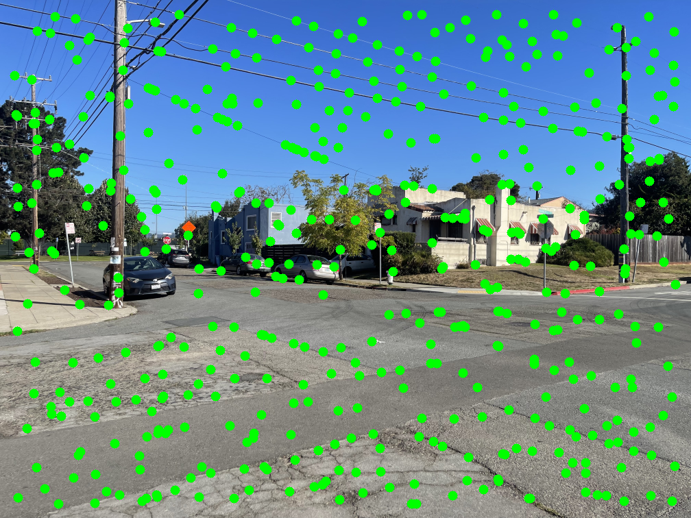
The middle image shows the resulting ANMS points, and the right image displays these points overlaid on the original Harris detections.

Part 2.2: Feature Descriptor Extraction

Implementation

Now that I have a set of points defining each image, the next step is to relate them across images. A single point doesn't contain enough information for comparison, but a small patch around it does. To do this, I iterate through all ANMS points from each image and extract a \( (40 \times 40) \) patch of pixels centered at each point.

Each patch is then downsampled to a size of \( (8 \times 8) \) to reduce memory usage and computation time while preserving coarse local structure. Finally, I normalize every patch to have a mean of 0 and a standard deviation of 1, making them invariant to changes in lighting. The image below shows several example features extracted using this process.

Part 2.3: Feature Mapping

Now that the features have been extracted from each image, the next step is to determine which patches correspond between them. For clarity, I'll refer to the two images as image1 and image2. To find correspondences, each feature in image1 is compared against all features in image2.

Each \(8 \times 8\) patch from the feature extraction stage is flattened into a 64-dimensional vector, allowing direct numerical comparison between features. The similarity between two features is measured using the Euclidean distance between their corresponding vectors.

A naive method would be to match each feature in image1 to its single closest feature in image2. However, this can easily produce incorrect matches, as the nearest feature might not represent the same structure.

A more reliable method is Lowe's ratio test. In this approach, the two closest features in image2 to a given feature in image1 are identified, and the ratio between their distances is computed. If the ratio is small, meaning one feature is much closer than the other, it indicates a stronger and more distinctive match. This method significantly reduces false correspondences while retaining true ones. In my implementation, I kept a match only if the ratio was below the threshold \( t=0.7 \). To improve performance, I used SciPy's cKDTree for efficient nearest-neighbor searches.

The image below shows several feature pairs between the two images. Although the pixel colors may differ, the structural patterns within each matched region are remarkably similar.

The images below show the marked points where features were matched. Notice that most points have a clear corresponding point in the other image.

Part 2.4: RANSAC for Robust Homography

Even with ANMS and feature matching, a few incorrect correspondences can still remain. Because least squares is highly sensitive to outliers, even a small number of bad matches can distort the entire homography computation. To address this, I applied RANdom SAmple Consensus (RANSAC), which effectively filters out most, if not all, of the incorrect matches.

RANSAC runs for a fixed number of iterations. For my images, I used 1000 iterations. In each iteration, four matching feature pairs are randomly selected to compute a homography. Using this homography, every feature in image1 is projected onto image2. The distance between each projected feature and its actual corresponding point in image2 is then measured. If the distance is below a threshold \( \epsilon \), that feature is added to the inlier set. In my implementation, I used \( \epsilon = 3\) pixels. After each iteration, the largest inlier set found so far is saved, and once all iterations are complete, the final inlier set is returned.

Using the points returned by RANSAC, I compute a refined homography and stitch the two images together using the warping and blending techniques described earlier.

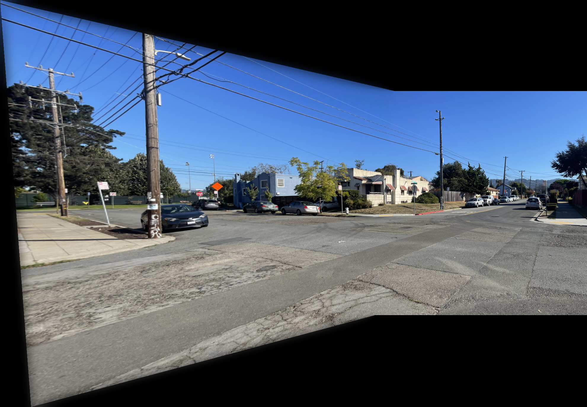
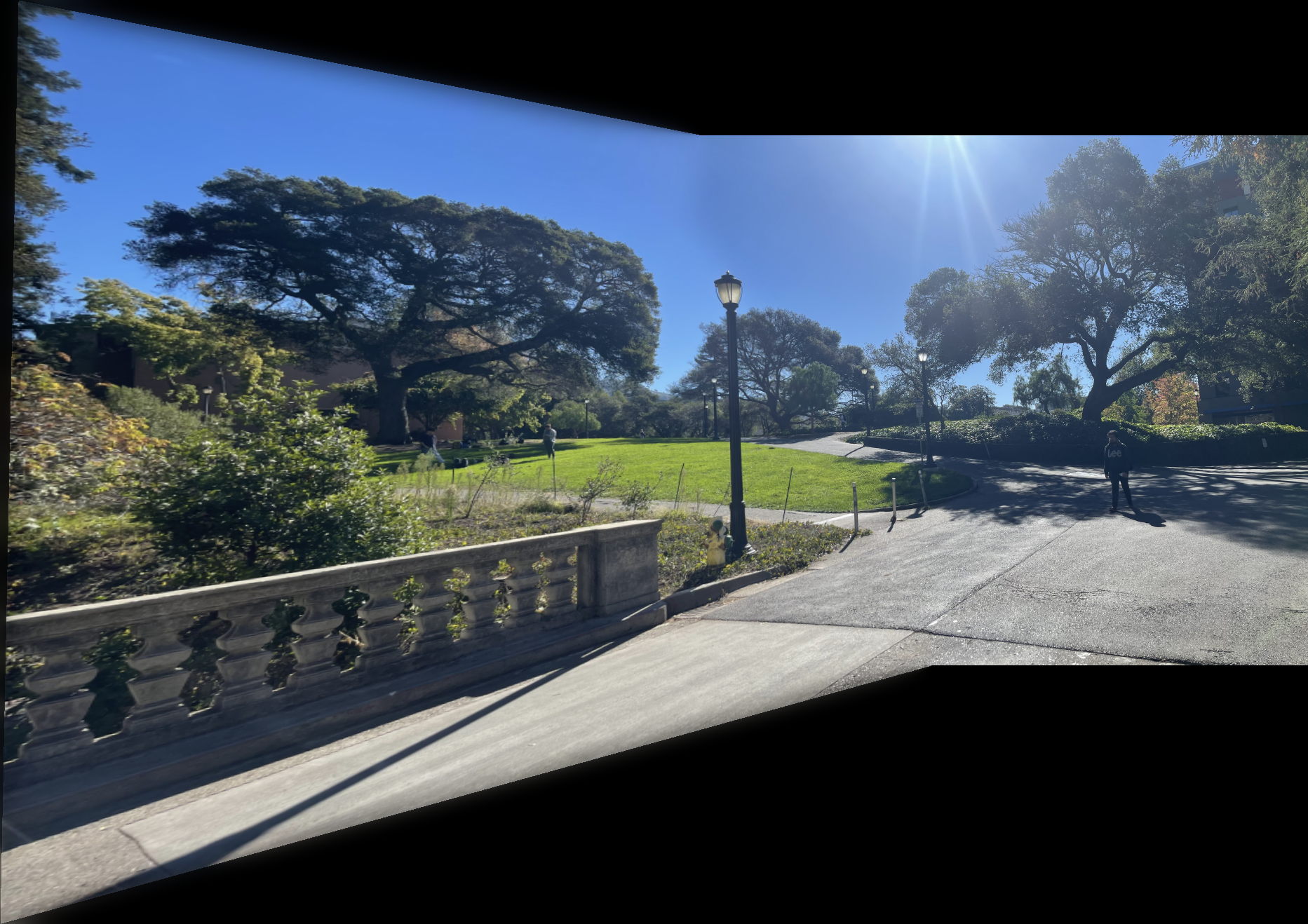
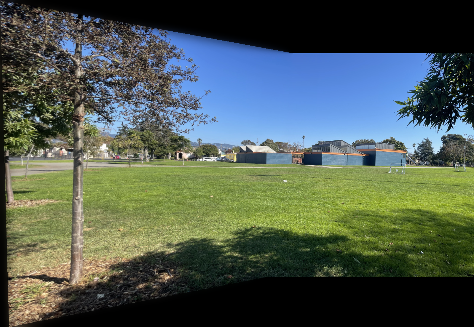
The images below show additional examples of autostitched results. On the left are images stitched using manually selected correspondence points, and on the right are images created through automatic stitching. I observed that the autostitched images appear less warped and slightly better.

Conclusion

Through this project, I implemented and analyzed key components of an image stitching pipeline, gaining a deeper understanding of how feature detection, matching, and transformation estimation interact to produce coherent panoramas. The resulting mosaics were generally sharp and well-aligned, with minor distortions caused by imperfect matches or perspective variation. Overall, this project reinforced the connection between mathematical models and practical computer vision systems used in applications like panorama generation and image registration.